Chapter 26: scikit-learn

Learning Objectives¶

By the end of this lecture, you will be able to:

Use scikit-learn to perform supervised learning
Understand the difference between classification and regression
Train and evaluate classification models
Train and evaluate regression models

`scikit-learn`¶

scikit-learn is a Python package that provides simple and efficient tools for data analysis. It is built on numpy, scipy, and matplotlib. It is open source and commercially usable under the BSD license. It is a great tool for machine learning in Python.

Installation¶

To install scikit-learn, you can follow the instructions on the official website. You can install it using pip:

pip install -U scikit-learn

Supervised Learning¶

In supervised learning, we have a dataset consisting of both input features and output labels. The goal is to learn a mapping from the input to the output. We have two types of supervised learning:

Classification: The output is a category.
Regression: The output is a continuous value.

Classification¶

In classification, we have a dataset consisting of input features and output labels. The goal is to learn a mapping from the input features to the output labels. We can use the scikit-learn library to perform classification.

Machine Learning by Example: Wine Classification¶

Let’s consider an example of wine classification. We have a dataset of wines with different features such as alcohol content, acidity, etc. We want to classify the wines into different categories based on these features.

Step 1: Get the Data¶

First, we need to load the dataset. We can use the load_wine function from sklearn.datasets to load the wine dataset.

import numpy as np
import pandas as pd
from sklearn.datasets import load_wine

data = load_wine()
df = pd.DataFrame(data.data, columns=data.feature_names)
df['target'] = data.target
df.head()

Step 2: Explore and Visualize the Data¶

Next, we need to explore and visualize the data to understand its structure and characteristics. We can use pandas to explore the data and seaborn to visualize it.

df.describe()

df['target'].value_counts()

target
1    71
0    59
2    48
Name: count, dtype: int64

import seaborn as sns
import matplotlib.pyplot as plt

sns.pairplot(df, hue='target')

plt.show()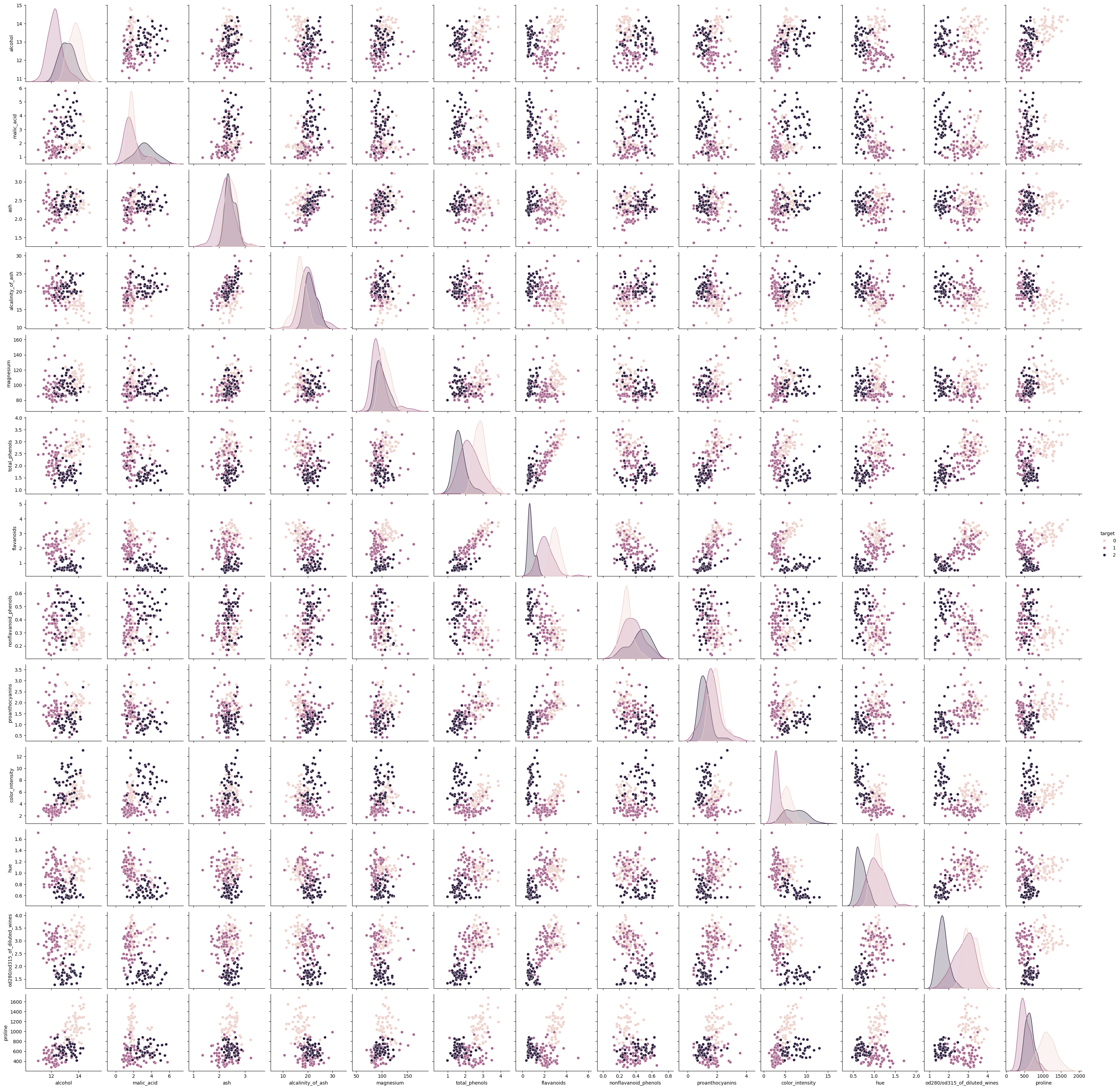

<Figure size 3308.87x3250 with 182 Axes>

Step 3: Preprocess the Data¶

Before training the model, we need to preprocess the data. This involves splitting the data into input features and output labels, normalizing the input features, and splitting the data into training and testing sets.

from sklearn.model_selection import train_test_split
from sklearn.preprocessing import StandardScaler

X = df.drop('target', axis=1)
y = df['target']

X_train, X_test, y_train, y_test = train_test_split(X, y, test_size=0.8, random_state=42)

scaler = StandardScaler()
X_train = scaler.fit_transform(X_train)
X_test = scaler.transform(X_test)

Step 4: Train a Model¶

Now that we have preprocessed the data, we can train a classification model. We will use the LogisticRegression and RandomForestClassifier models from scikit-learn.

from sklearn.linear_model import LogisticRegression
from sklearn.ensemble import RandomForestClassifier
from sklearn.metrics import ConfusionMatrixDisplay
import matplotlib.pyplot as plt

# Train the Logistic Regression model
lr = LogisticRegression()
lr.fit(X_train, y_train)
y_pred_lr = lr.predict(X_test)

# Train the Random Forest model
rf = RandomForestClassifier()
rf.fit(X_train, y_train)
y_pred_rf = rf.predict(X_test)

# Plot the confusion matrix
fig, ax = plt.subplots(1, 2, figsize=(12, 6))
ConfusionMatrixDisplay.from_estimator(lr, X_test, y_test, ax=ax[0])
ax[0].set_title('Logistic Regression')
ConfusionMatrixDisplay.from_estimator(rf, X_test, y_test, ax=ax[1])
ax[1].set_title('Random Forest')

plt.show()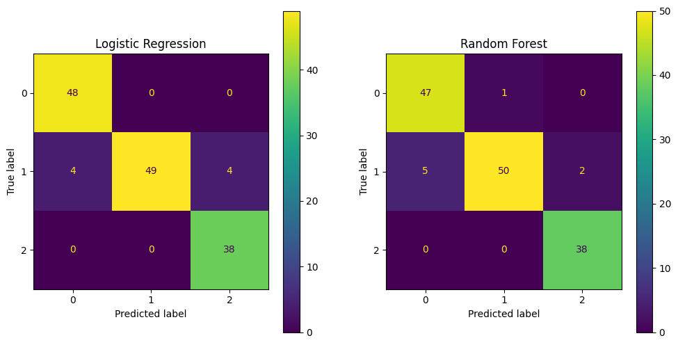

Step 5: Evaluate the Model¶

Finally, we need to evaluate the model’s performance. We can use metrics such as accuracy, precision, recall, and F1 score to evaluate the model.

from sklearn.metrics import classification_report

print('Logistic Regression:')
print(classification_report(y_test, y_pred_lr))

print('Random Forest:')
print(classification_report(y_test, y_pred_rf))

Logistic Regression:
              precision    recall  f1-score   support

           0       0.92      1.00      0.96        48
           1       1.00      0.86      0.92        57
           2       0.90      1.00      0.95        38

    accuracy                           0.94       143
   macro avg       0.94      0.95      0.94       143
weighted avg       0.95      0.94      0.94       143

Random Forest:
              precision    recall  f1-score   support

           0       0.94      0.98      0.96        48
           1       0.98      0.91      0.95        57
           2       0.95      1.00      0.97        38

    accuracy                           0.96       143
   macro avg       0.96      0.96      0.96       143
weighted avg       0.96      0.96      0.96       143

Classification Report

A classification report shows the precision, recall, F1 score, and support for each class in the classification model. Precision is the ratio of true positives to the sum of true positives and false positives

\text{Precision} = \frac{\text{True Positives}}{\text{True Positives} + \text{False Positives}}

(1)

Recall is the ratio of true positives to the sum of true positives and false negatives

\text{Recall} = \frac{\text{True Positives}}{\text{True Positives} + \text{False Negatives}}

(2)

The F1 score is the harmonic mean of precision and recall

F1 = 2 \times \frac{\text{Precision} \times \text{Recall}}{\text{Precision} + \text{Recall}}

(3)

Support is the number of occurrences of each class in the dataset.

Step 6: Plot and Interpret the Coefficients¶

For the logistic regression model, we can plot and interpret the coefficients to understand the importance of each feature in the classification.

import numpy as np

# Ensure feature names are a NumPy array
feature_names = np.array(data.feature_names)

# Sort the coefficients
sorted_idx = lr.coef_[0].argsort()

# Plot the coefficients
plt.figure(figsize=(12, 6))
plt.barh(feature_names[sorted_idx], lr.coef_[0][sorted_idx])
plt.xlabel('Coefficient Value')
plt.ylabel('Feature Name')
plt.title('Logistic Regression Coefficients')
plt.show()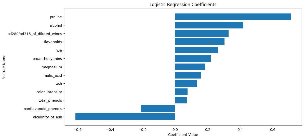

The plot above shows the coefficients of the logistic regression model. The features with the largest coefficients (in absolute value) are the most important for the classification. The sign of the coefficient indicates the direction of the relationship between the feature and the target. The two features with the largest coefficients are proline and alcalinity_of_ash.

proline is the amount of proline in the wine. Proline is an amino acid that is found in high concentrations in red wines. The coefficient for proline is positive, indicating that wines with higher proline content are more likely to be classified as class 2.

Figure 1:The chemical structure of proline. By Qohelet12, CC0, via Wikimedia Commons

alcalinity_of_ash is the amount of ash in the wine. Ash is the inorganic residue remaining after the water and organic matter have been removed by heating. The coefficient for alcalinity_of_ash is negative, indicating that wines with lower ash content are more likely to be classified as class 2.

Regression¶

In regression, we have a dataset consisting of input features and continuous output values. The goal is to learn a mapping from the input features to the output values. We can use the scikit-learn library to perform regression.

Machine Learning by Example: Oxygen Vacancy Formation Energy Prediction¶

Let’s consider an example of regression for predicting the oxygen vacancy formation energy in materials. We have an Excel file containing the features of the materials and the oxygen vacancy formation energy. We want to train a regression model to predict the oxygen vacancy formation energy based on the features of the materials.

Step 1: Use `pip` or `conda` to Install `openpyxl`¶

Before we can read the Excel file, we need to install the openpyxl library. You can install it using pip:

pip install openpyxl

Step 2: Get the Data¶

First, we need to load the dataset. We can use the pd.read_excel function from pandas to load the Excel file.

df = pd.read_excel('ovfe-deml.xlsx')
df.head()

Step 3: Explore and Visualize the Data¶

Next, we need to explore and visualize the data to understand its structure and characteristics. We can use pandas to explore the data and seaborn to visualize it.

Missing Values¶

Before exploring the data, we need to check for missing values and handle them if necessary.

df.isnull().sum()

xtal_str         0
comp             0
dHf              0
Eg_exp           9
Eg_GW            0
Eg_DFTU          0
O2p_min_VBM      0
dEN              0
OVFE_calc        0
OVFE_reg_GW      0
OVFE_reg_DFTU    0
Ehull_MP         2
dtype: int64

The measured band gap (Eg_exp) and the energy above the convex hull (Ehull_MP) have nine and two missing values, respectively. We can drop these columns or impute the missing values with the mean, median, or mode of the column. Let’s drop the columns for now.

df.drop(['Eg_exp', 'Ehull_MP'], axis=1, inplace=True)
df.head()

Data Exploration¶

Now, let’s explore the data to understand its structure and characteristics.

df.describe()

sns.pairplot(df, kind='reg', diag_kind='kde')
plt.show()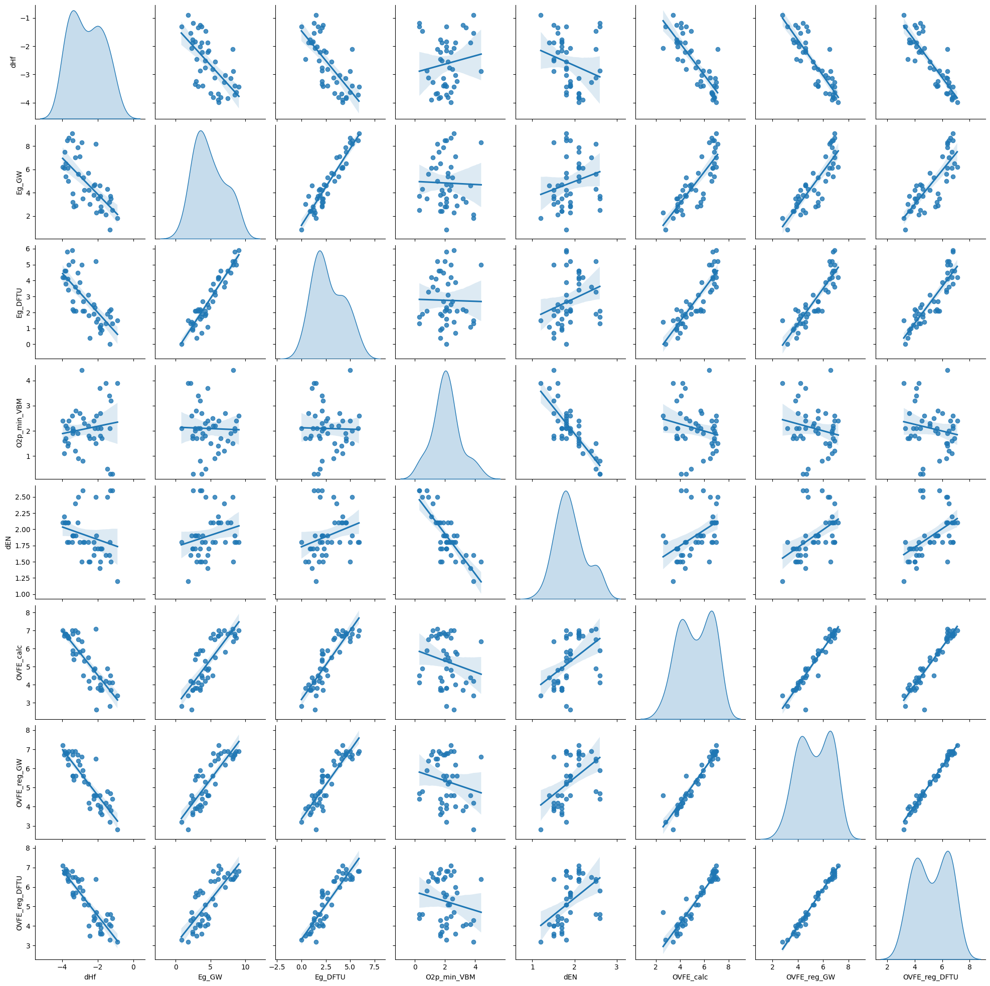

Step 4: Preprocess the Data¶

X = df.drop(['xtal_str', 'comp', 'OVFE_calc', 'OVFE_reg_GW', 'OVFE_reg_DFTU'], axis=1)
y = df['OVFE_calc']

X_train, X_test, y_train, y_test = train_test_split(X, y, test_size=0.2, random_state=42)

scaler = StandardScaler()
X_train = scaler.fit_transform(X_train)
X_test = scaler.transform(X_test)

Step 5: Train a Model¶

Now that we have preprocessed the data, we can train a regression model. We will use the RidgeCV and Perceptron models from scikit-learn.

from sklearn.linear_model import RidgeCV
from sklearn.neural_network import MLPRegressor

# Train the Ridge regression model
ridge = RidgeCV()
ridge.fit(X_train, y_train)
y_pred_ridge = ridge.predict(X_test)

# Train the MLPRegressor model
mlp = MLPRegressor(
    hidden_layer_sizes=(100, 50),
    activation='relu',
    solver='adam',
    max_iter=1000,
    random_state=42
)
mlp.fit(X_train, y_train)
y_pred_mlp = mlp.predict(X_test)

# Plot the predicted vs. actual values
plt.figure(figsize=(6, 6))
plt.scatter(y_test, y_pred_ridge, label='Ridge')
plt.scatter(y_test, y_pred_mlp, label='MLP')
plt.plot([min(y_test), max(y_test)], [min(y_test), max(y_test)], 'k--')
plt.xlabel('Actual Oxygen Vacancy Formation Energy (eV)')
plt.ylabel('Predicted Oxygen Vacancy Formation Energy (eV)')
plt.legend()
plt.show()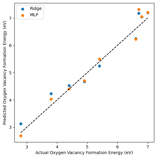

Step 6: Evaluate the Model¶

Finally, we need to evaluate the model’s performance. We can use metrics such as mean squared error (MSE), mean absolute error (MAE), and $R^2$ score to evaluate the model.

from sklearn.metrics import mean_squared_error, mean_absolute_error, r2_score

print('Ridge Regression:')
print('MSE:', mean_squared_error(y_test, y_pred_ridge))
print('MAE:', mean_absolute_error(y_test, y_pred_ridge))
print('R^2:', r2_score(y_test, y_pred_ridge))

print('MLPRegressor:')
print('MSE:', mean_squared_error(y_test, y_pred_mlp))
print('MAE:', mean_absolute_error(y_test, y_pred_mlp))
print('R^2:', r2_score(y_test, y_pred_mlp))

Ridge Regression:
MSE: 0.09159773749651347
MAE: 0.2804229419845595
R^2: 0.954743096637687
MLPRegressor:
MSE: 0.08291662572137232
MAE: 0.23271115977294177
R^2: 0.9590322881332733

Regression Metrics

Mean squared error (MSE) is the average of the squared differences between the predicted and actual values

\text{MSE} = \frac{1}{n} \sum_{i=1}^{n} (y_i - \hat{y}_i)^2

(4)

Mean absolute error (MAE) is the average of the absolute differences between the predicted and actual values

\text{MAE} = \frac{1}{n} \sum_{i=1}^{n} |y_i - \hat{y}_i|

(5)

The $R^2$ score is the coefficient of determination and represents the proportion of the variance in the dependent variable that is predictable from the independent variables

R^2 = 1 - \frac{\sum_{i=1}^{n} (y_i - \hat{y}_i)^2}{\sum_{i=1}^{n} (y_i - \bar{y})^2}

(6)

Step 7: Plot and Interpret the Coefficients¶

For the Ridge regression model, we can plot and interpret the coefficients to understand the importance of each feature in the regression.

# Ensure feature names are a NumPy array
feature_names = np.array(X.columns)

# Sort the coefficients
sorted_idx = ridge.coef_.argsort()

# Plot the coefficients
plt.figure(figsize=(12, 6))
plt.barh(feature_names[sorted_idx], ridge.coef_[sorted_idx])
plt.xlabel('Coefficient Value')
plt.ylabel('Feature Name')
plt.title('Ridge Regression Coefficients')
plt.show()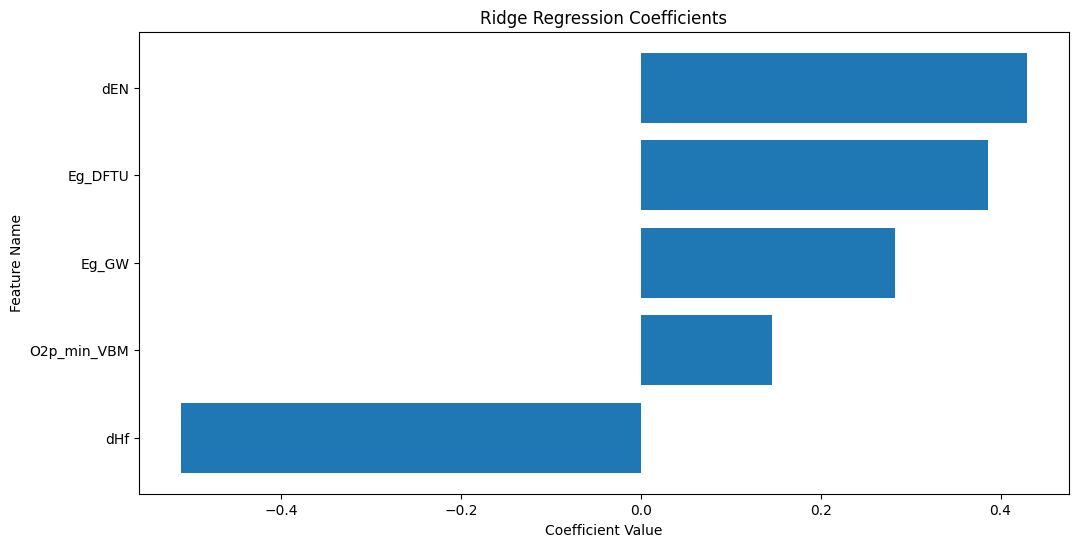

The plot above shows the coefficients of the Ridge regression model. The features with the largest coefficients (in absolute value) are the most important for the regression. The sign of the coefficient indicates the direction of the relationship between the feature and the target. The feature with the largest coefficient is dHf.

Summary¶

In this lecture, we learned how to use scikit-learn to perform supervised learning. We covered classification and regression and trained models on the wine recognition dataset and the oxygen vacancy formation energy dataset. We explored the data, preprocessed it, trained the models, evaluated the models, and interpreted the results. We used logistic regression and random forests for classification and ridge regression and MLPRegressor for regression. We also visualized the data, plotted the confusion matrix, and interpreted the coefficients.

References¶

Deml, A. M., Holder, A. M., O’Hayre, R. P., Musgrave, C. B., & Stevanović, V. (2015). Intrinsic Material Properties Dictating Oxygen Vacancy Formation Energetics in Metal Oxides. The Journal of Physical Chemistry Letters, 6(10), 1948–1953. 10.1021/acs.jpclett.5b00710

Part 7. Advanced and Emerging Topics in Computational Chemistry

Chapter 25: Kinetic Monte Carlo