1.1. Course Introduction

Overview and Learning Objectives¶

Thermodynamics and statistical mechanics connect microscopic models of matter to macroscopic observables such as temperature, pressure, and free energy. This section introduces course conventions, the language of systems and surroundings, and the role of state variables in equilibrium descriptions. It also reviews common forms of energy, energy transfer, and the unit conventions used throughout the course.

This course develops the core concepts of thermodynamics and statistical mechanics and applies them to chemical systems. It builds on the thermodynamic principles introduced in Chem 106 and Chem 112, and on the quantum mechanics developed in Chem 105, Chem 111, and Chem 401. By connecting molecular-level behavior to macroscopic thermodynamic observations, you will see how theory underpins real-world chemical processes.

Learning objectives:

Define system, surroundings, and boundary; distinguish isolated/closed/open systems.
Distinguish state variables/state functions from process-dependent (path) quantities, and explain what makes a quantity a state function.
State the criteria for mechanical/thermal/chemical equilibrium used to justify thermodynamic state descriptions.
Convert between common thermodynamic units (Pa, bar, atm; J, kJ, eV; K and °C) and check dimensional consistency.

Core Ideas and Derivations¶

Why Study Thermodynamics and Statistical Mechanics?¶

Bridging the Microscopic and Macroscopic Worlds¶

Typical chemical systems contain on the order of Avogadro’s number of particles (i.e., $N_{\mathrm{A}} = 6.022 \times 10^{23}$ ). Thermodynamics abstracts this complexity into a framework for predicting, among other things,

reaction spontaneity,
equilibrium states, and
phase transitions.

Modern Applications¶

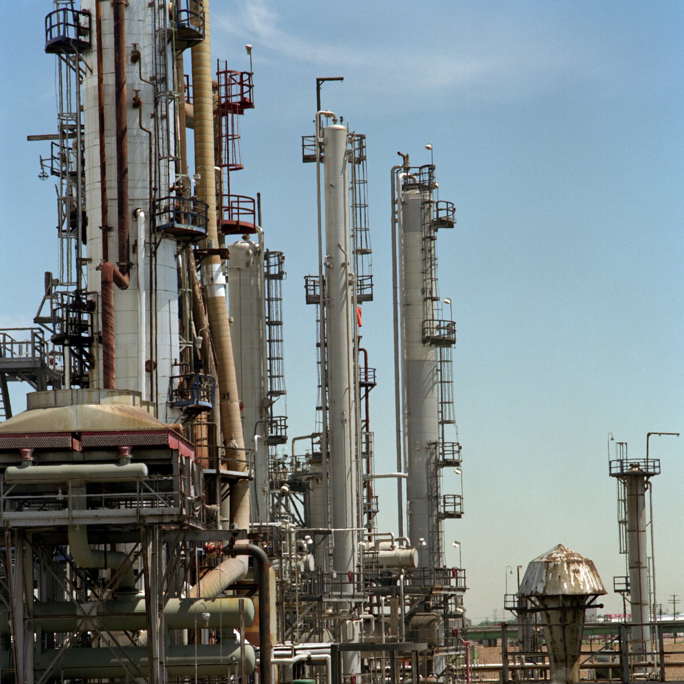
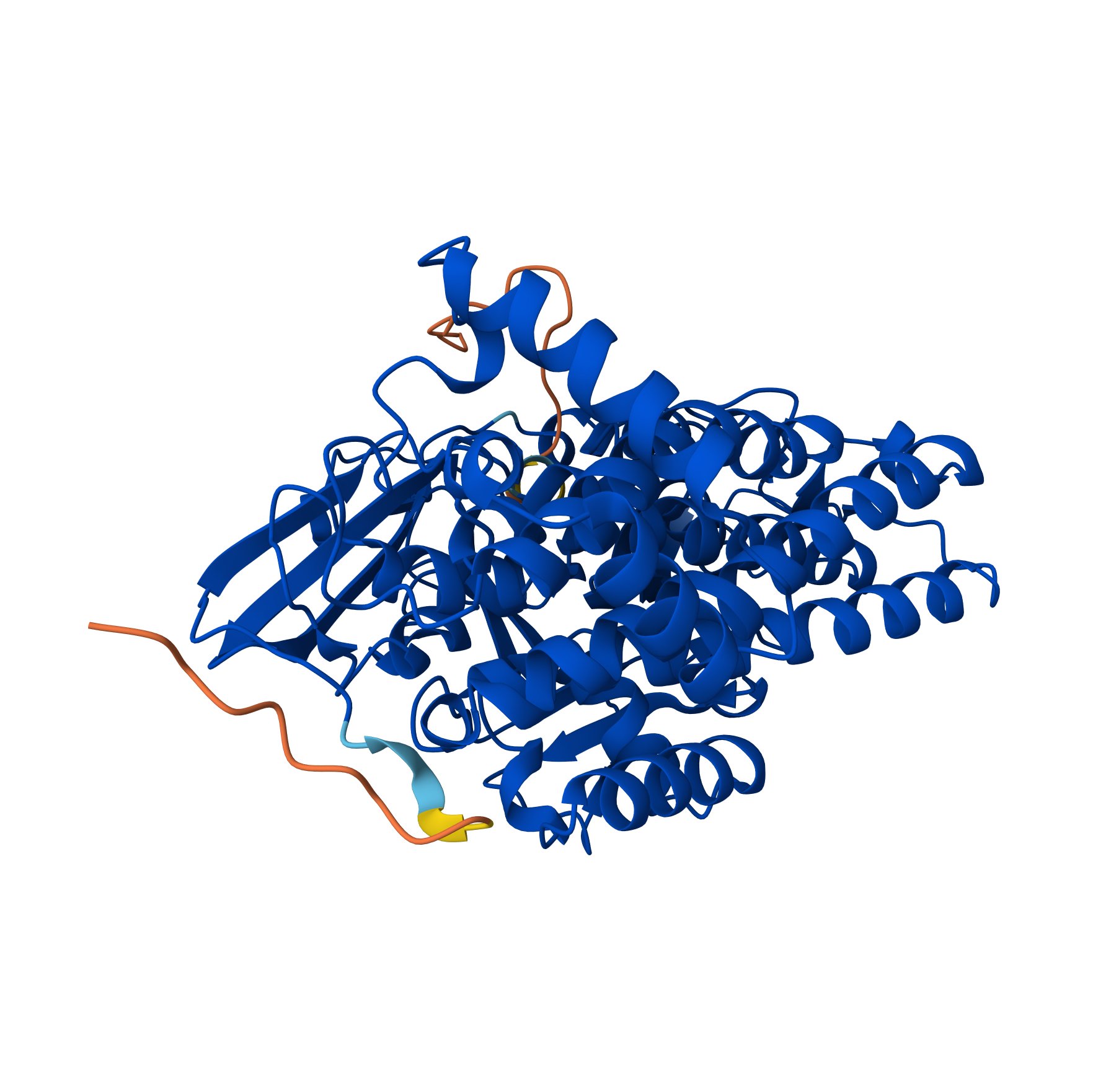
Thermodynamics and statistical mechanics are central to diverse fields, including industrial chemistry, materials science, and biochemistry. The examples below illustrate a few representative applications:

Industrial Chemistry

Predicting reaction spontaneity and modeling large-scale chemical processes.

Figure 1:Hydrogen production via steam–methane reforming.^[1]

Materials Chemistry

Designing advanced materials for optical, electronic, or mechanical applications.

Figure 2:Electricity generation using solar panels.^[2]

Biochemistry

Investigating protein folding and enzyme activity in biological systems.

Figure 3:Predicting protein structures with AlphaFold.^[3]

Key Definitions¶

Thermodynamic Systems¶

import matplotlib.pyplot as plt
import matplotlib.patches as mpatches
from myst_nb import glue

# Helper function to plot a system
def plot_system(ax, title, annotations, boundary_color='b'):
    box = mpatches.FancyBboxPatch((0, 0), 1, 1, boxstyle='roundtooth', ec=boundary_color, fc='w')
    ax.add_patch(box)
    ax.set_title(title, fontsize=14)
    ax.text(0.5, 0.5, 'System', ha='center', va='center', fontsize=12)
    ax.text(0.5, -0.65, 'Surroundings', ha='center', va='center', fontsize=12)
    ax.text(0.5, 1.3, 'Boundary', ha='center', va='bottom', fontsize=12, color=boundary_color)
    for annotation in annotations:
        if "arrowprops" in annotation:  # Arrow annotations
            ax.annotate('', **annotation)
        else:  # Text annotations
            ax.text(**annotation)
    ax.set_xlim(-1, 2)
    ax.set_ylim(-1, 2)
    ax.set_aspect('equal')
    ax.axis('off')

# Define annotations for each system
annotations = [
    [],  # Isolated system (no arrows)
    [  # Closed system (energy arrow)
        dict(xy=(-0.6, 0.15), xytext=(0.15, 0.15), arrowprops=dict(arrowstyle='<->', color='r')),
        dict(x=-1, y=0.3, s='Energy', ha='left', va='bottom', fontsize=12, color='r'),
    ],
    [  # Open system (energy + matter arrows)
        dict(xy=(-0.6, 0.15), xytext=(0.15, 0.15), arrowprops=dict(arrowstyle='<->', color='r')),
        dict(xy=(0.85, 0.15), xytext=(1.6, 0.15), arrowprops=dict(arrowstyle='<->', color='m')),
        dict(x=-1, y=0.3, s='Energy', ha='left', va='bottom', fontsize=12, color='r'),
        dict(x=2, y=0.3, s='Matter', ha='right', va='bottom', fontsize=12, color='m'),
    ],
]

titles = ["Isolated system", "Closed system", "Open system"]

fig, axes = plt.subplots(1, 3, figsize=(12, 4))
for i, ax in enumerate(axes):
    plot_system(ax, titles[i], annotations[i])

plt.show()
plt.close(fig)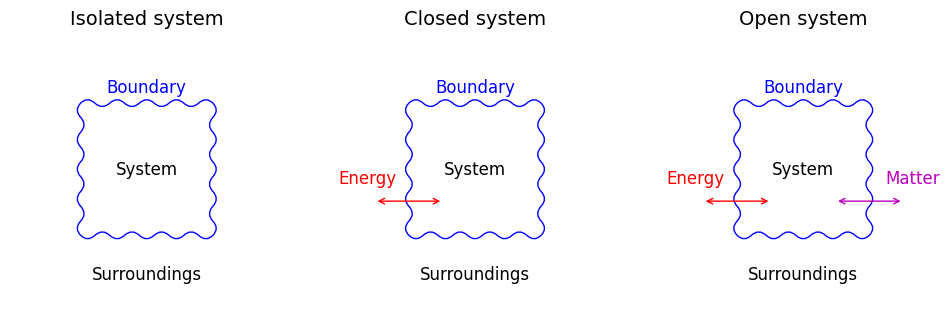

Types of thermodynamic systems. (a) Isolated—no exchange of energy or matter; (b) Closed—exchanges energy but not matter; (c) Open—exchanges both energy and matter.

System: The portion of the universe chosen for study, separated from its surroundings by a boundary.
Surroundings: Everything external to the system that can exchange energy or matter with it.
Boundary: The interface separating a system from its surroundings.
Isolated system: Exchanges neither energy nor matter with its surroundings.
Closed system: Exchanges energy but not matter with its surroundings.
Open system: Exchanges both energy and matter with its surroundings.

State of a System¶

Particle: A microscopic entity such as an atom, molecule, or ion.
Microscopic state (classical): Positions and momenta of all particles in the system.
Microscopic state (quantum): The wavefunction describing the system’s particles.
Equilibrium: A condition in which macroscopic properties remain constant over time.
Thermodynamic equilibrium: Simultaneous mechanical, thermal, and chemical equilibrium.
Thermodynamic state: A set of macroscopic variables defining a system in equilibrium.
State variable: A property that defines a system’s state.
State function: A property depending only on the system’s state, not on the path taken.
Equation of state: A mathematical relationship among state variables.
Path function: A property depending on the process or path taken between states.
Process: A transformation changing a system from one state to another.
Extensive property: A property proportional to system size (e.g., volume, entropy).
Intensive property: A property independent of system size (e.g., temperature, pressure).

Basic Forms of Energy and Energy Transfer¶

Energy¶

Kinetic energy: Energy due to motion (e.g., a moving particle).
Potential energy: Energy due to position or configuration (e.g., a stretched spring).
Internal energy: The total microscopic kinetic and potential energy of a system, averaged over its microstates.

Energy Transfer¶

Work: Energy transferred when a force acts over a distance (e.g., lifting a mass).
Heat: Energy transferred because of a temperature difference (e.g., conduction from hot to cold).

Important Units¶

SI Units^[4]¶

Table 1:Base SI Units

Quantity	Unit	Symbol
Time	second	s
Length	meter	m
Mass	kilogram	kg
Temperature	kelvin	K

Table 2:Derived SI Units

Quantity	Unit	Symbol	Conversion
Frequency	hertz	Hz	$1 \,\text{Hz} = 1 \,\text{s}^{-1}$
Force	newton	N	$1 \,\text{N} = 1 \,\text{kg m s}^{-2}$
Pressure	pascal	Pa	$1 \,\text{Pa} = 1 \,\text{N m}^{-2}$
Energy	joule	J	$1 \,\text{J} = 1 \,\text{N m}$

Non-SI Units^[5]^[6]^[7]¶

Table 3:Non-SI Units

Quantity	Unit	Symbol	Conversion
Pressure	bar	bar	$1 \,\text{bar} = 1 \times 10^5 \,\text{Pa}$
Pressure	atmosphere	atm	$1 \,\text{atm} \approx 1.01325 \,\text{bar}$
Pressure	torr	torr	$1 \,\text{torr} = \frac{1}{760}\,\text{atm}$
Pressure	millimeters of mercury	mmHg	$1 \,\text{mmHg} = 1 \,\text{torr}$
Energy	electronvolt	eV	$1 \,\text{eV} = 1.602 \times 10^{-19} \,\text{J}$
Energy	calorie	cal	$1 \,\text{cal} = 4.184 \,\text{J}$

Worked Example¶

Unit conversions you will use constantly¶

A gas sample has pressure $P=1.50\ \mathrm{atm}$ at $T=25.0^{\circ}\mathrm{C}$ . Convert $P$ to bar and Pa, and convert $T$ to kelvin.

Assumptions. Use $1\ \mathrm{atm}=1.01325\times 10^{5}\ \mathrm{Pa}$ and $1\ \mathrm{bar}=10^{5}\ \mathrm{Pa}$ .

Temperature to kelvin
$T(\mathrm{K}) = T(^{\circ}\mathrm{C}) + 273.15 \quad\Rightarrow\quad T = 25.0 + 273.15 = 298.15\ \mathrm{K}.$
(1)
Pressure to pascals
$P = (1.50\ \mathrm{atm})\left(1.01325\times 10^{5}\ \frac{\mathrm{Pa}}{\mathrm{atm}}\right) = 1.52\times 10^{5}\ \mathrm{Pa}.$
(2)
Pressure to bar
$P = \frac{1.52\times 10^{5}\ \mathrm{Pa}}{10^{5}\ \mathrm{Pa/bar}} = 1.52\ \mathrm{bar}.$
(3)

Result. $T=298.15\ \mathrm{K}$ , $P=1.52\times10^{5}\ \mathrm{Pa}=1.52\ \mathrm{bar}$ .

Concept Checks¶

Why does thermodynamics emphasize state functions rather than path-dependent quantities?
Give one real-world example each of an isolated, closed, and open system. What crosses the boundary in each case?
Which variables would you choose as “independent” to describe a gas in a rigid, sealed container? In a piston open to the atmosphere?
Why is dimensional analysis a useful error-checking tool in thermodynamic derivations?

Key Takeaways¶

Thermodynamics models macroscopic behavior using a small set of state variables together with equilibrium assumptions.
Systems are classified by what they exchange across the boundary: energy, matter, or neither.
State functions depend only on the state, not the path; unit consistency is non-negotiable.
Clear notation and unit conventions reduce errors and make derivations reusable across topics.

Footnotes¶