1.2. Kinetic Theory - Physical Chemistry II

Overview and Learning Objectives¶

Kinetic theory provides a microscopic route to macroscopic gas behavior by modeling a gas as a large number of rapidly moving particles that undergo elastic collisions. In this section, we derive the pressure of an ideal gas from particle–wall momentum transfer, connect temperature to average kinetic energy, and interpret molecular speed distributions.

Learning objectives:

List the assumptions of kinetic theory used to model an ideal gas.
Derive the relation $P=\tfrac{1}{3}(N/V)m\langle v^{2}\rangle$ from particle–wall momentum transfer.
Use $\langle E_{\mathrm{kin}}\rangle = \tfrac{3}{2}k_{\mathrm{B}}T$ to relate temperature to molecular motion.
Compute characteristic speeds ( $v_{\mathrm{mp}},\ \langle v\rangle,\ v_{\mathrm{rms}}$ ) and interpret the Maxwell–Boltzmann distribution.

Core Ideas and Derivations¶

Foundational Assumptions of Kinetic Theory¶

Large Number of Particles:
A gas contains a very large number of identical particles moving randomly in all directions.
Point Particles:
Each particle’s size is negligible compared to the average distance between particles.
Elastic Collisions:
Collisions between particles and between particles and the container walls conserve both momentum and kinetic energy.
No Long-Range Interparticle Forces:
Particles exert no forces on one another except during collisions (i.e., there are no long-range attractive or repulsive forces).
Classical Mechanics Applies:
Particle motion follows Newton’s second law:
$\vec{F} = \frac{d\vec{p}}{dt},$
(1)
where $\vec{F}$ is the net force on a particle, $\vec{p}$ is its linear momentum, and $t$ is time.

Deriving Pressure from Particle-Wall Collisions¶

import matplotlib.pyplot as plt
from myst_nb import glue

def plot_container_2d(offset=0.2):
    """Plot a 2D schematic of a gas particle in a container."""
    fig, ax = plt.subplots(figsize=(12, 4))

    # Dimensions
    Lx, Lz = 10, 2

    # Draw container
    ax.plot([0, Lx, Lx, 0, 0], [0, 0, Lz, Lz, 0], color='black')
    ax.fill_between([0, Lx], 0, Lz, color='lightgray')

    # Gas particle
    ax.plot(0.5 * Lx, 0.75 * Lz, 'o', color='blue', markersize=20, zorder=10)
    ax.text(0.5 * Lx, 0.75 * Lz, "$m$", color='white',
            ha='center', va='center', zorder=20, fontsize=12)

    # Velocity arrows
    ax.annotate("", xy=(0.5 * Lx, 0.75 * Lz), xytext=(Lx, 0.75 * Lz),
                arrowprops=dict(arrowstyle="<-", color='red'))
    ax.text(Lx * 2 / 3, 0.75 * Lz + offset, "$v_x$", color='red', fontsize=12, ha='center', va='center')

    ax.annotate("", xy=(Lx, 0.5 * Lz), xytext=(0, 0.5 * Lz),
                arrowprops=dict(arrowstyle="<-", color='red'))
    ax.text(Lx * 5 / 6, 0.5 * Lz + offset, "$-v_x$", color='red', fontsize=12, ha='center', va='center')

    ax.annotate("", xy=(0, 0.25 * Lz), xytext=(0.5 * Lx, 0.25 * Lz),
                arrowprops=dict(arrowstyle="<-", color='red'))
    ax.text(0.25 * Lx, 0.25 * Lz + offset, "$v_x$", color='red', fontsize=12, ha='center', va='center')

    # Length indicators
    ax.annotate("", xy=(0, -offset), xytext=(Lx, -offset),
                arrowprops=dict(arrowstyle="<->", color='black'))
    ax.text(Lx / 2, -2 * offset, "$L_x$", color='black', fontsize=12, ha='center', va='center')

    ax.annotate("", xy=(-offset, 0), xytext=(-offset, Lz),
                arrowprops=dict(arrowstyle="<->", color='black'))
    ax.text(-2 * offset, Lz / 2, "$L_z$", color='black', fontsize=12, ha='center', va='center')

    ax.set_xlim(-1, Lx+1)
    ax.set_ylim(-1, Lz+1)
    ax.axis('off')

    return fig

fig = plot_container_2d()
plt.show()
plt.close(fig)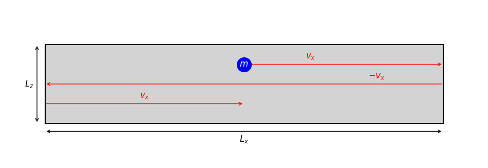

Two-dimensional schematic of a single gas particle in a cuboid container (gray). Velocity components are shown in red. The length $L_y$ is not depicted, as it extends perpendicular to the plane of view.

Microscopic Picture of Pressure¶

Pressure is the force exerted per unit area on the container walls. Microscopically, it arises from momentum transfer during particle–wall collisions.

Particle Momentum Change¶

Consider an elastic collision of a particle of mass $m$ with a wall perpendicular to the $x$ -axis. The $x$ -component of the velocity reverses ( $v_x \to -v_x$ ). If we take $v_x>0$ to denote the magnitude of the $x$ -component, then the magnitude of the particle’s momentum change is

\Delta p_x = 2 m v_x.

(2)

Time Between Collisions¶

If the container has length $L_x$ in the $x$ -direction, the time between successive collisions of the same particle with that wall is

\Delta t = \frac{2 L_x}{v_x}.

(3)

Force on the Wall¶

A single particle’s average force on the wall (in the $x$ -direction) is then

F_{\text{p}, x} = \frac{\Delta p_x}{\Delta t} = \frac{m v_x^2}{L_x}.

(4)

Total Pressure¶

For $N$ identical particles with isotropic motion in a volume $V$ , the total pressure $P$ is

P = \frac{1}{V} \sum_{i=1}^N \frac{1}{3} m v_i^2,

(5)

where $v_i$ is the speed of the $i$ -th particle. Using the mean-square speed $\langle v^2 \rangle$ , we obtain

P = \frac{N m \langle v^2 \rangle}{3 V}.

(6)

This equation shows how macroscopic pressure depends on the microscopic particle speeds.

Kinetic Energy and Temperature¶

The average translational kinetic energy per particle is

\langle E_{\mathrm{kin}} \rangle = \frac{1}{2} m \langle v^2 \rangle.

(7)

Equating Eq. (6) with the ideal-gas equation of state, $PV = N k_{\mathrm{B}} T$ (discussed in Section 3), gives

\frac{1}{2} m \langle v^2 \rangle = \frac{3}{2} k_{\mathrm{B}} T,

(8)

where $k_{\mathrm{B}}$ is the Boltzmann constant and $T$ is the absolute temperature. This result—often presented as an application of equipartition—shows that temperature is directly proportional to the average translational kinetic energy of the particles.

Complete Derivation of the Relationship Between Kinetic Energy and Temperature

1. Kinetic Energy of a Single Particle
Consider a single particle with mass $m$ and speed $v$ . Its translational kinetic energy is

E_{\text{p},\,\mathrm{kin}} \;=\; \frac{1}{2}\,m\,v^{2}.

(9)

2. Total Kinetic Energy of $N$ Particles
For $N$ particles with masses $m_1, m_2, \ldots, m_N$ and respective speeds $v_1, v_2, \ldots, v_N$ , the total translational kinetic energy is

E_{\mathrm{kin}}\left(m_1,\ldots,m_N\right) \;=\; \frac{1}{2}\,\sum_{i=1}^{N} m_i\,v_i^2.

(10)

If all particles are identical with mass $m$ , this simplifies to

E_{\mathrm{kin}} \;=\; \frac{1}{2}\,m\,\sum_{i=1}^{N} v_i^2.

(11)

3. Defining the Average of the Speed Squared
Define the mean-square speed

\langle v^2 \rangle \;=\; \frac{1}{N}\,\sum_{i=1}^{N} v_i^2,

(12)

so that

\sum_{i=1}^{N} v_i^2 \;=\; N\,\langle v^2 \rangle.

(13)

Substituting back gives

4. Relating Pressure to Kinetic Energy
From Eq. (6), the pressure $P$ in a volume $V$ can be written as

P \;=\; \frac{N\,m\,\langle v^2 \rangle}{3\,V}.

(15)

Recognizing that $N m \langle v^2 \rangle / 2 = E_{\mathrm{kin}}$ , we obtain

P \;=\; \frac{2\,E_{\mathrm{kin}}}{3\,V}.

(16)

5. Equating to the Ideal-Gas Equation of State
For an ideal gas (discussed in Section 3),

P \;=\; \frac{N\,k_{\mathrm{B}}\,T}{V}.

(17)

Equating the two expressions for $P$ ,

\frac{2\,E_{\mathrm{kin}}}{3\,V} \;=\; \frac{N\,k_{\mathrm{B}}\,T}{V},

(18)

and solving for $E_{\mathrm{kin}}$ gives

E_{\mathrm{kin}} \;=\; \frac{3}{2}\,N\,k_{\mathrm{B}}\,T.

(19)

6. Average Kinetic Energy Per Particle (Equipartition Theorem)
Dividing by $N$ yields the average kinetic energy per particle:

Each translational degree of freedom contributes $k_{\mathrm{B}}T/2$ to the average kinetic energy.

Maxwell–Boltzmann Speed Distribution¶

The rms speed $v_{\mathrm{rms}}$ is a useful single-number summary, but in thermal equilibrium a gas has a distribution of particle speeds.

For an ideal gas in three dimensions, the Maxwell–Boltzmann speed distribution gives the probability density $f(v)$ for finding a molecule with speed between $v$ and $v+dv$ :

f(v) = 4\pi\left(\frac{m}{2\pi k_{\mathrm{B}}T}\right)^{3/2} v^2\,\exp\!\left(-\frac{m v^2}{2k_{\mathrm{B}}T}\right), \qquad v\ge 0.

(21)

It is normalized so that $\int_0^\infty f(v)\,dv = 1$ .

Most probable speed and mean speed¶

From $f(v)$ we can define several “typical” speeds:

v_{\mathrm{mp}} = \sqrt{\frac{2k_{\mathrm{B}}T}{m}} \qquad \text{(speed at the peak of } f(v)\text{)}

(22)

\langle v\rangle = \int_0^\infty v\,f(v)\,dv = \sqrt{\frac{8k_{\mathrm{B}}T}{\pi m}}.

(23)

The rms speed is

v_{\mathrm{rms}} = \sqrt{\langle v^2\rangle} = \sqrt{\frac{3k_{\mathrm{B}}T}{m}}.

(24)

For any Maxwell–Boltzmann distribution, these satisfy

v_{\mathrm{mp}} < \langle v\rangle < v_{\mathrm{rms}}.

(25)

Comparing gases and temperatures¶

The Maxwell–Boltzmann curves below illustrate two trends:

Lighter gases (smaller $m$ ) have distributions shifted to higher speeds.
Higher temperatures shift the distribution to higher speeds and make it broader.

import numpy as np
import matplotlib.pyplot as plt
from scipy.constants import k as k_B, N_A


def f_MB(v, M_kg_per_mol, T):
    """Maxwell–Boltzmann speed distribution f(v) for an ideal gas.

    Parameters
    ----------
    v : array
        Speeds (m/s).
    M_kg_per_mol : float
        Molar mass (kg/mol).
    T : float
        Temperature (K).

    Returns
    -------
    f : array
        Probability density (s/m).
    """
    m = M_kg_per_mol / N_A  # mass per molecule (kg)
    prefactor = 4 * np.pi * (m / (2 * np.pi * k_B * T)) ** 1.5
    return prefactor * v**2 * np.exp(-m * v**2 / (2 * k_B * T))


# Molar masses (kg/mol)
M_He = 4.002602e-3
M_N2 = 28.0134e-3
M_CO2 = 44.0095e-3

cases = [
    (M_CO2, 300, r"CO$_2$ (300 K)"),
    (M_N2, 300, r"N$_2$ (300 K)"),
    (M_N2, 600, r"N$_2$ (600 K)"),
    (M_He, 300, r"He (300 K)"),
]

v = np.linspace(0, 4000, 4000)

fig, ax = plt.subplots(figsize=(6, 4))

for M, T, label in cases:
    ax.plot(v, f_MB(v, M, T), label=label)

ax.set_xlabel("Speed $v$ (m/s)")
ax.set_ylabel(r"Probability density $f(v)$")
ax.set_xlim(0, 4000)
ax.grid(True)
ax.legend(frameon=False)

plt.tight_layout()
plt.show()
plt.close(fig)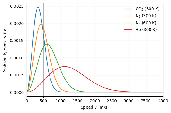

Maxwell–Boltzmann speed distributions for different gases and temperatures.

Worked Example¶

Root-mean-square speed at room temperature¶

Estimate the rms speed of $\mathrm{N_2}$ molecules at $T=300\ \mathrm{K}$ .

Assumptions. Ideal-gas kinetic theory and equipartition; $v_{\mathrm{rms}}=\sqrt{3k_{\mathrm{B}}T/m}$ .
Take $m(\mathrm{N_2}) = 28.0\,u = 28.0(1.66054\times10^{-27})\ \mathrm{kg} = 4.65\times10^{-26}\ \mathrm{kg}$ .

Insert numbers
$v_{\mathrm{rms}}=\sqrt{\frac{3k_{\mathrm{B}}T}{m}} =\sqrt{\frac{3(1.38065\times10^{-23}\ \mathrm{J/K})(300\ \mathrm{K})}{4.65\times10^{-26}\ \mathrm{kg}}}.$
(26)
Evaluate
$v_{\mathrm{rms}}=\sqrt{2.67\times10^{5}\ \mathrm{m^2/s^2}} \approx 5.17\times10^{2}\ \mathrm{m/s}.$
(27)

Result. $v_{\mathrm{rms}}(\mathrm{N_2},300\ \mathrm{K})\approx 5.2\times10^{2}\ \mathrm{m/s}$ .

Concept Checks¶

Which kinetic-theory assumption is most directly violated at high pressures or low temperatures?
Why does pressure depend on $\langle v_x^2\rangle$ (or $\langle v^2\rangle$ ) rather than on $\langle v_x\rangle$ ?
How would doubling the absolute temperature change $v_{\mathrm{rms}}$ ?
What physical information is encoded in the width of the Maxwell–Boltzmann speed distribution?

Key Takeaways¶

Pressure arises from momentum transfer during particle–wall collisions.
For an ideal gas, temperature measures average translational kinetic energy.
Characteristic molecular speeds scale as $\sqrt{T/m}$ .
The Maxwell–Boltzmann distribution explains why gases contain a range of speeds even at fixed $T$ .