1.3. Ideal Gases

See also: Course-wide Conventions & Notation

Overview and Learning Objectives¶

The ideal-gas model consolidates several empirical gas laws into a single equation of state and is accurate when intermolecular interactions are negligible. In this section, we review the classical gas laws, derive $PV=Nk_{\mathrm{B}}T=nRT$, use the result to estimate microscopic length scales, and see how it motivates an absolute temperature scale.

Learning objectives:

• State Boyle’s, Charles’s, Gay–Lussac’s, and Avogadro’s laws and identify the variables held constant in each.

• Derive the ideal-gas equation of state $PV=Nk_{\mathrm{B}}T=nRT$ by combining the gas laws.

• Explain the microscopic assumptions behind ideal-gas behavior and when they are expected to hold.

• Use $V/N=(k_{\mathrm{B}}T/P)$ to estimate number density and mean intermolecular spacing.

Core Ideas and Derivations¶

Gas Laws¶

Source

import matplotlib.pyplot as plt
import numpy as np
from scipy.constants import k, N_A
from labellines import labelLines
from myst_nb import glue

# Constants
T = 290  # Temperature in Kelvin (Boyle's Law)
P = 1.0  # Fixed pressure in bar (Charles' Law)
V = 24.53  # Fixed volume in liters (Gay-Lussac's Law)
N = N_A   # Number of particles for Avogadro's Law

temperatures = np.linspace(273.15, 373.15, 101)   # Temperatures in Kelvin
volumes = np.linspace(1, 40, 400)  # Volumes in liters
number_of_particles = np.linspace(0.1, 10, 100) * N_A

# Calculate pressures, volumes, etc., according to each law
pressures_boyle = N * k * T / volumes * 0.01
volumes_charles = (N * k / P * 0.01) * temperatures
pressures_gay_lussac = (N * k / V) * temperatures * 0.01
volumes_avogadro = (k * T / P * 0.01) * number_of_particles

def plot_law(ax, x, y, label, title, xlabel, ylabel):
    line = ax.plot(x, y, "b-", label=label)
    ax.set_title(title, fontsize=14)
    ax.set_xlabel(xlabel, fontsize=12)
    ax.set_ylabel(ylabel, fontsize=12)
    ax.grid(True, linestyle="--", linewidth=0.5)
    labelLines(line, zorder=2.5)

fig, axs = plt.subplots(1, 4, figsize=(12, 3))

# Boyle's Law
plot_law(axs[0], volumes, pressures_boyle, "$P = c_\\text{B} / V$", "Boyle (1662)",
         "Volume (L)", "Pressure (bar)")
axs[0].text(0.1, 0.9, 'Constant $T$ & $N$', transform=axs[0].transAxes)

# Charles's Law
plot_law(axs[1], temperatures, volumes_charles, "$V = c_\\text{C} T$", "Charles (1787)",
         "Temperature (K)", "Volume (L)")
axs[1].text(0.1, 0.9, 'Constant $P$ & $N$', transform=axs[1].transAxes)

# Gay-Lussac's Law
plot_law(axs[2], temperatures, pressures_gay_lussac, "$P = c_\\text{GL} T$", "Gay-Lussac (1802)",
         "Temperature (K)", "Pressure (bar)")
axs[2].text(0.1, 0.9, 'Constant $V$ & $N$', transform=axs[2].transAxes)

# Avogadro's Law
plot_law(axs[3], number_of_particles / N_A, volumes_avogadro, "$V = c_\\text{A} N$", "Avogadro (1811)",
         "Number of Particles ($N_{\\mathrm{A}}$)", "Volume (L)")
axs[3].text(0.1, 0.9, 'Constant $P$ & $T$', transform=axs[3].transAxes)

plt.tight_layout()
plt.show()
plt.close(fig)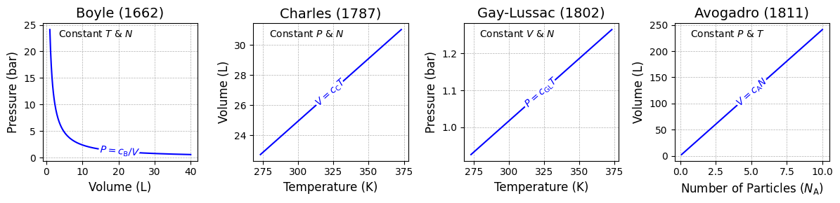

Four classical gas laws (blue), shown in chronological order: Boyle’s law^[1], Charles’s law, Gay–Lussac’s law, and Avogadro’s law.

Real gases approximately follow these relationships when at least one of the following conditions is met:

• pressure is relatively low,

• density is relatively low, and/or

• temperature is sufficiently high.

These conditions collectively minimize intermolecular interactions, allowing the gas to behave ideally.

Deriving an Equation of State¶

In Section 1, we defined an equation of state as a mathematical relationship among state variables. Each gas law above relates two state variables (among $P, V, T, N$) under conditions where the other two are held constant. To obtain a single equation of state relating all four variables, we can combine these laws using multivariate calculus (as covered in Math 233).

Total Differential¶

The total differential $df$ of a function $f$ of $m$ variables $x_1, \ldots, x_m$ is

where $\left(\partial f / \partial x_i\right)_{\{ x_j | j \neq i \}}$ denotes the partial derivative of $f$ with respect to $x_i$, holding all other variables constant, and $dx_i$ is an infinitesimal change in $x_i$.

Total Differential of Volume¶

From Boyle’s, Charles’s, and Avogadro’s laws, we can treat $V$ as a function of $P, T,$ and $N$:

Applying Eq. (1) to $V$ gives

Partial Derivatives via Gas Laws¶

Using the gas laws in differential form, one finds

Dividing by $V$ and rearranging (i.e., using logarithmic differentials) yields

Integrating the Total Differential¶

Integrating from an initial state $(P_i, V_i, T_i, N_i)$ to a final state $(P_f, V_f, T_f, N_f)$ gives

Because the initial and final states are arbitrary, the ratio $PV/(NT)$ must be a constant. Denoting this constant by $k_{\mathrm{B}}$, we arrive at the ideal-gas equation of state:

where $n = N / N_{\mathrm{A}}$ is the number of moles and $R = k_{\mathrm{B}} N_{\mathrm{A}}$ is the molar gas constant ($R = 8.314\,\mathrm{J\,mol^{-1}\,K^{-1}}$).

Ideal-Gas Assumptions¶

A gas described by Eq. (7) is called ideal because, under low pressures, low densities, or high temperatures, we can adopt the simplifying assumptions of kinetic theory:

1. Particles have negligible volume (point particles).

2. Particles experience no intermolecular forces except during elastic collisions.

3. Collisions conserve total energy and momentum.

Many thermodynamic properties follow cleanly from these assumptions.

Estimating Particle Distances¶

Rearranging Eq. (7), a simple estimate for a typical intermolecular spacing is

This expression shows that increasing temperature or reducing pressure increases the typical separation between gas particles.

Absolute Temperature Scale¶

Source

import matplotlib.pyplot as plt
import numpy as np
import pandas as pd
from scipy.constants import N_A
import statsmodels.api as sm
from myst_nb import glue

# Experimental data for O2 at 1 Pa:
df = pd.read_table("../_static/section-03/isobaric-properties-for-oxygen.tsv", sep="\t").iloc[:, [0, 1, 3]]
df.columns = ["T_C", "P", "V"]
df["v"] = df["V"] * 1e27 / N_A  # Convert volume to nm³/molecule

X = sm.add_constant(df["v"])  # For intercept in linear regression
y = df["T_C"]
model = sm.OLS(y, X).fit()

df["T_C_pred"] = model.predict(X)

fig, ax = plt.subplots(figsize=(4, 4))
ax.plot(df["v"], df["T_C"], "b.")
intercept, slope = model.params
line = ax.plot(df["v"], df["T_C_pred"], "r-", label=f"Slope: {slope:.2e}; Intercept: {intercept:.2f} °C")
labelLines(line, zorder=2.5)

ax.set_xlabel("Volume (nm³/molecule)")
ax.set_ylabel("Temperature (°C)")
ax.grid(True, linestyle="--", linewidth=0.5)

plt.tight_layout()
plt.show()
plt.close(fig)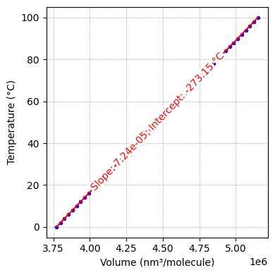

Linear relationship between the per-molecule volume $v$ and Celsius temperature for O₂ at 1 Pa.^[2]
The red line is an ordinary least-squares fit; its intercept at $-273.15\,{}^{\circ}\mathrm{C}$ corresponds to the extrapolated zero-volume limit and therefore to absolute zero (0 K).

Charles’s law states that, at constant (sufficiently low) pressure, the volume per particle is directly proportional to the gas temperature. If temperature is reported on the Celsius scale ($0\,{}^{\circ}\mathrm{C}$ at the freezing point of water and $100\,{}^{\circ}\mathrm{C}$ at the boiling point), plotting $v$ versus $T(\,{}^{\circ}\mathrm{C})$ gives an approximately linear relationship. Extrapolating this line to the (unphysical) point where the volume would vanish identifies a theoretical lower bound at $-273.15\,{}^{\circ}\mathrm{C}$. Shifting the Celsius scale by 273.15 degrees places this bound at zero:

This defines the Kelvin scale, an absolute temperature scale that begins at the lowest physically meaningful temperature.

Worked Example¶

Mean intermolecular spacing at 1 bar¶

Estimate the mean spacing $\langle d\rangle$ between molecules in an ideal gas at $T=300\ \mathrm{K}$ and $P=1.00\ \mathrm{bar}$.

Using

with $k_{\mathrm{B}}=1.38065\times10^{-23}\ \mathrm{J/K}$ and $P=1.00\times10^{5}\ \mathrm{Pa}$:

1. Compute $k_{\mathrm{B}}T/P$

   $$\frac{k_{\mathrm{B}}T}{P}=\frac{(1.38065\times10^{-23})(300)}{1.00\times10^{5}} =4.14\times10^{-26}\ \mathrm{m^3}.$$

   (11)

2. Take the cube root

   $$\langle d\rangle=(4.14\times10^{-26})^{1/3} \approx 3.46\times10^{-9}\ \mathrm{m} =3.46\ \mathrm{nm}.$$

   (12)

Result. At $300\ \mathrm{K}$ and $1\ \mathrm{bar}$, molecules are typically separated by a few nanometers.

Concept Checks¶

1. Why does the ratio $PV/(NT)$ have to be constant if the total-differential argument holds for arbitrary initial/final states?

2. Which change (increasing $T$ or increasing $P$) makes a gas less ideal, and why?

3. Why must temperature be measured on an absolute (Kelvin) scale in the ideal-gas law?

4. How would $\langle d\rangle$ scale if pressure increased by a factor of 8 at fixed $T$?

Key Takeaways¶

• The classical gas laws combine into the ideal-gas equation of state $PV=Nk_{\mathrm{B}}T=nRT$.

• Ideal behavior is expected at low density/pressure or high temperature, where interactions are small.

• The mean molecular spacing scales as $\langle d\rangle\propto (T/P)^{1/3}$.

• The Kelvin scale emerges naturally because the gas-law proportionalities require $T>0$ and linearity in $T$.