1.4. Real Gases

Overview and Learning Objectives¶

Real gases deviate from ideal behavior when finite molecular size and intermolecular forces become important. This section introduces the compressibility factor as a quantitative measure of nonideality and develops the van der Waals equation of state (EOS), including its critical constants and the principle of corresponding states.

At sufficiently high pressures (high densities) or low temperatures, we can no longer treat gases as collections of noninteracting point particles. High pressure/density brings molecules closer together, increasing collision frequency and making both excluded volume and intermolecular interactions more consequential. Lower temperature reduces kinetic energy, so these interactions more strongly perturb $PVT$ behavior. This section develops practical ways to quantify deviations from ideality and introduces the van der Waals EOS—one of the simplest real-gas models and the work recognized by the Nobel Prize in Physics 1910.

Learning objectives:

Define the compressibility factor $Z$ and interpret $Z<1$ vs. $Z>1$ in terms of net attractions/repulsions.
Write the van der Waals EOS in particle and molar forms and interpret the parameters $a$ and $b$ .
Derive (or use) the van der Waals critical constants $V_{\mathrm m,c}=3b$ , $P_c=a/(27b^2)$ , $T_c=8a/(27bR)$ .
Non-dimensionalize the van der Waals EOS to obtain the corresponding-states form in reduced variables.

Core Ideas and Derivations¶

Deviations from Ideal Behavior¶

Compressibility Factor¶

import matplotlib.pyplot as plt
import numpy as np
import pandas as pd
from scipy.constants import R
from labellines import labelLines
from myst_nb import glue
from scipy.interpolate import interp1d

# Load the experimental data for water at 300 K
df = pd.read_csv("../_static/section-04/isothermal-properties-for-water-T=300.csv").iloc[:, [0, 1, 2, 3]]
df.columns = ["T", "P", "rho_m", "V_m"]  # Rename columns

# Calculate the compressibility factor
df["P_Pa"] = df["P"] * 1e5  # Convert pressure from bar to Pa
df["Z"] = df["P_Pa"] * df["V_m"] / (R * df["T"])

# Set up figure and axis
fig, ax = plt.subplots(figsize=(4, 4))
ax.set_xlim(0, 1000)
ax.set_ylim(0, 2)
ax.set_xlabel("Pressure (bar)")
ax.set_ylabel(r"$Z$")
ax.grid(True, linestyle="--", alpha=0.7)

# Plot experimental compressibility factor
data_line = ax.plot(df["P"], df["Z"], "b-", label="$Z_\\text{water}$")
labelLines(data_line, xvals=[400], zorder=2.5)

# Plot ideal gas line
x_values = np.linspace(0, 1000, 100)
ideal_line = ax.plot(x_values, np.ones_like(x_values), "r--", label="$Z_\\text{ideal}$")
labelLines(ideal_line, xvals=[400], zorder=2.5)

# Interpolate to find intersection with ideal gas line
interp_Z = interp1d(df["P"], df["Z"], kind='linear', fill_value="extrapolate")
intersection_pressure = interp1d(df["Z"] - 1, df["P"], kind='linear')(0)
intersection_Z = interp_Z(intersection_pressure)

# Find pressure and Z value at minimum Z
min_Z_index = df["Z"].idxmin()
min_pressure = df.loc[min_Z_index, "P"]
min_Z = df.loc[min_Z_index, "Z"]

# Annotate ideal and coincidentally ideal points
ax.annotate("Ideal",
            xy=(0, 1), xytext=(200, 1.25),
            arrowprops=dict(arrowstyle="->"),
            ha='center', va='center', zorder=4)

ax.annotate("Coincidentally\nideal",
            xy=(intersection_pressure, 1), xytext=(800, 0.75),
            arrowprops=dict(arrowstyle="->"),
            ha='center', va='center', zorder=4)

# Draw vertical lines for reference
ax.axvline(x=min_pressure, color="black", linestyle=":")
ax.axvline(x=intersection_pressure, color="black", linestyle=":")

# Highlight regions of attractive and repulsive behavior
ax.fill_between([min_pressure, intersection_pressure], 0, 2, color="magenta", alpha=0.2, label="Attractive")
ax.fill_between([intersection_pressure, 1000], 0, 2, color="gray", alpha=0.2, label="Repulsive")

# Annotate regions
x_values_for_attractive = np.linspace(min_pressure, intersection_pressure, 100)
attractive_line = ax.plot(x_values_for_attractive, np.ones_like(x_values_for_attractive) * min_Z, "m-", label="Attractive", alpha=0.0)
labelLines(attractive_line, xvals=np.mean([min_pressure, intersection_pressure]), zorder=2.5)

x_values_for_repulsive = np.linspace(intersection_pressure, 1000, 100)
repulsive_line = ax.plot(x_values_for_repulsive, np.ones_like(x_values_for_repulsive) * min_Z, "gray", label="Repulsive", alpha=0.0)
labelLines(repulsive_line, xvals=800, zorder=2.5)

# Adjust layout and display
plt.tight_layout()
plt.show()
plt.close(fig)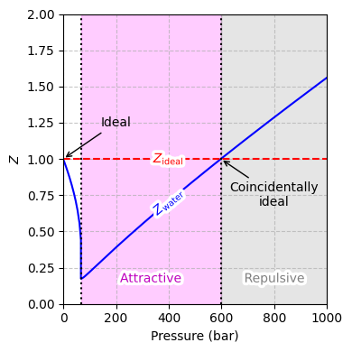

Compressibility factor $Z$ for water at 300 K as a function of pressure, with the ideal-gas line ( $Z=1$ ) included for comparison. The dip below $Z=1$ indicates net attractive forces (most pronounced at the minimum in $Z$ ), while the rise above $Z=1$ at higher pressures reflects repulsive interactions. The intersection with $Z=1$ marks a “coincidentally ideal” state.

One convenient measure of nonideality is the compressibility factor $Z$ :

Z = \frac{P V}{N k_\text{B} T} = \frac{P V}{n R T}.

(1)

Table 1:Behavior of Water at Different Pressures

Pressure	$Z$	Volume	Analysis	Water
High	$> 1$	$V_\text{real} > V_\text{ideal}$	Repulsive interactions	Pauli (steric) repulsion
Medium	$< 1$	$V_\text{real} < V_\text{ideal}$	Attractive interactions	H-bonding and van der Waals interactions
Low	$= 1$	$V_\text{real} = V_\text{ideal}$	Ideal-gas behavior	—

Van der Waals Fluid¶

Van der Waals Equation of State¶

The van der Waals equation of state is among the simplest real-gas models (and was central to the work recognized by the Nobel Prize in Physics 1910):

Table 2:Forms of the van der Waals Equation of State

	Extensive Volume	Intensive Volume
Per Particle	$\left( P + \frac{a_\text{p} N^2}{V^2} \right) \left( V - b_\text{p} N \right) = N k_\text{B} T$ (2)	$\left( P + \frac{a_\text{p}}{V_\text{p}^2} \right) \left( V_\text{p} - b_\text{p} \right) = k_\text{B} T$ (3)
Per Mole	$\left( P + \frac{a_\text{m} n^2}{V^2} \right) \left( V - b_\text{m} n \right) = n R T$ (4)	$\left( P + \frac{a_\text{m}}{V_\text{m}^2} \right) \left( V_\text{m} - b_\text{m} \right) = R T,$ (5)

where $a$ and $b$ are substance-dependent parameters capturing two departures from ideality:

$a$ : Net attractive interactions between particles.
$b$ : Volume associated with finite particle size (excluded volume).

Van der Waals Isotherm¶

import matplotlib.pyplot as plt
from matplotlib.lines import Line2D
import numpy as np
import pandas as pd
from scipy.constants import R
from labellines import labelLines
from myst_nb import glue

# van der Waals constants for carbon dioxide
a_m_L_bar = 3.6551  # L^2 bar / mol^2
b_m_L = 0.042816  # L / mol
L_to_m3 = 1e-3  # m^3 / L
bar_to_Pa = 1e5  # Pa / bar
a_m = a_m_L_bar * L_to_m3**2 * bar_to_Pa  # m^6 Pa / mol^2
b_m = b_m_L * L_to_m3  # m^3 / mol

# van der Waals critical properties for carbon dioxide
Tc_vdW = 8 * a_m / (27 * b_m * R)  # K
Pc_vdW = a_m / (27 * b_m**2)  # Pa
Vc_vdW = 3 * b_m  # m^3 / mol

# Experimental phase change data for carbon dioxide
Tc_exp = 304.18  # K
Pc_exp = 73.80 * bar_to_Pa  # Pa
Vc_exp = 0.0919 * L_to_m3  # m^3 / mol

# van der Waals pressure function
def van_der_waals_pressure(a, b, T, V):
    return R * T / (V - b) - a / V**2

# Load experimental data
def load_experimental_data(filename):
    df = pd.read_csv(filename).iloc[:, [0, 1, 2, 3]]
    df.columns = ["Tc", "P", "rho_m", "V_m"]
    return df

df_lt_Tc = load_experimental_data("../_static/section-04/isothermal-properties-for-carbon-dioxide-Tr=0.9.csv")
df_at_Tc = load_experimental_data("../_static/section-04/isothermal-properties-for-carbon-dioxide-Tr=1.0.csv")
df_gt_Tc = load_experimental_data("../_static/section-04/isothermal-properties-for-carbon-dioxide-Tr=1.1.csv")

# Set up figure
fig, ax = plt.subplots(figsize=(4, 4))
Vm_vdW = np.linspace(0.5 * Vc_vdW, 20 * Vc_vdW, 1000)

# Plot van der Waals isotherms
colors = ["b", "r", "m"]
temps = [0.9 * Tc_vdW, Tc_vdW, 1.1 * Tc_vdW]
labels = ["$T < T_c$", "$T = T_c$", "$T > T_c$"]
lines = []
for T, color, label in zip(temps, colors, labels):
    P_vdW = van_der_waals_pressure(a_m, b_m, T, Vm_vdW)
    line = ax.plot(Vm_vdW / L_to_m3, P_vdW / bar_to_Pa, color + "-", label=label)
    lines.append(line)
    labelLines(line, xvals=[0.3], zorder=2.5)

# Plot experimental isotherms
for df, color in zip([df_lt_Tc, df_at_Tc, df_gt_Tc], colors):
    ax.plot(df["V_m"] / L_to_m3, df["P"], color + "-", alpha=0.5)

# Legend and labels
legend_elements = [Line2D([0], [0], c='k', label='van der Waals', ls="-"),
                   Line2D([0], [0], c='k', label='Experimental', ls="-", alpha=0.5)]
ax.set_xlim(0, 1)
ax.set_ylim(0, 100)
ax.set_xlabel("Molar Volume (L/mol)")
ax.set_ylabel("Pressure (bar)")
ax.legend(handles=legend_elements, loc='lower left')
ax.grid(True, linestyle="--", alpha=0.7)

# Adjust layout and display
plt.tight_layout()
plt.show()
plt.close(fig)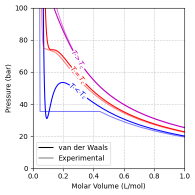

Comparison of experimental and van der Waals isotherms for CO $_2$ at temperatures below, at, and above the critical temperature $T_c$ . For $T < T_c$ , the van der Waals EOS exhibits the characteristic loop associated with phase separation; at $T = T_c$ the isotherm has an inflection point; and for $T > T_c$ the liquid–vapor transition disappears.

Critical Point¶

# Reference: https://scipython.com/blog/the-maxwell-construction/

import numpy as np
import pandas as pd
import matplotlib.pyplot as plt
from matplotlib.lines import Line2D
from scipy.constants import R as R_SI
from scipy.integrate import quad
from scipy.optimize import curve_fit, newton
from scipy.signal import argrelextrema
from scipy import stats
from labellines import labelLines
from myst_nb import glue

R = R_SI / 100  # Gas constant in L bar / mol K

# van der Waals constants for carbon dioxide
a_m = 3.6551    # L^2 bar/mol^2
b_m = 0.042816  # L/mol

# van der Waals critical properties for carbon dioxide
Tc_vdW = 8 * a_m / (27 * b_m * R)  # K
Pc_vdW = a_m / (27 * b_m**2)       # bar
Vc_vdW = 3 * b_m                   # L/mol

# Reduced-pressure form of the van der Waals equation of state
def vdw(Tr, Vr):
    """Van der Waals equation of state.

    Return the reduced pressure from the reduced temperature and volume.

    """

    pr = 8*Tr/(3*Vr-1) - 3/Vr**2
    return pr

# Maxwell construction of the reduced-pressure form of the van der Waals equation of state
def vdw_maxwell(Tr, Vr):
    """Van der Waals equation of state with Maxwell construction.

    Return the reduced pressure from the reduced temperature and volume,
    applying the Maxwell construction correction to the unphysical region
    if necessary.

    """

    pr = vdw(Tr, Vr)
    if Tr >= 1:
        # No unphysical region above the critical temperature.
        return pr

    if min(pr) < 0:
         raise ValueError('Negative pressure results from van der Waals'
                         ' equation of state with Tr = {} K.'.format(Tr))

    # Initial guess for the position of the Maxwell construction line:
    # the volume corresponding to the mean pressure between the minimum and
    # maximum in reduced pressure, pr.
    iprmin = argrelextrema(pr, np.less)
    iprmax = argrelextrema(pr, np.greater)
    Vr0 = np.mean([Vr[iprmin], Vr[iprmax]])

    def get_Vlims(pr0):
        """Solve the inverted van der Waals equation for reduced volume.

        Return the lowest and highest reduced volumes such that the reduced
        pressure is pr0. It only makes sense to call this function for
        T<Tc, ie below the critical temperature where there are three roots.

        """

        eos = np.poly1d( (3*pr0, -(pr0+8*Tr), 9, -3) )
        roots = eos.r
        roots.sort()
        Vrmin, _, Vrmax = roots
        return Vrmin, Vrmax

    def get_area_difference(Vr0):
        """Return the difference in areas of the van der Waals loops.

        Return the difference between the areas of the loops from Vr0 to Vrmax
        and from Vrmin to Vr0 where the reduced pressure from the van der Waals
        equation is the same at Vrmin, Vr0 and Vrmax. This difference is zero
        when the straight line joining Vrmin and Vrmax at pr0 is the Maxwell
        construction.

        """

        pr0 = vdw(Tr, Vr0)
        Vrmin, Vrmax = get_Vlims(pr0)
        return quad(lambda vr: vdw(Tr, vr) - pr0, Vrmin, Vrmax)[0]

    # Root finding by Newton's method determines Vr0 corresponding to
    # equal loop areas for the Maxwell construction.
    Vr0 = newton(get_area_difference, Vr0)
    pr0 = vdw(Tr, Vr0)
    Vrmin, Vrmax = get_Vlims(pr0)

    # Set the pressure in the Maxwell construction region to constant pr0.
    pr[(Vr >= Vrmin) & (Vr <= Vrmax)] = pr0
    return pr, Vrmin, Vrmax

# Reduced volume range
Vr = np.linspace(0.5, 20, 1000)

fig, axs = plt.subplot_mosaic([[0, 1]], figsize=(8, 4), sharex=True, sharey=True)

# Plot the van der Waals isotherm below the critical temperature
line1 = axs[0].plot(Vr * Vc_vdW,
                    vdw(0.9, Vr) * Pc_vdW,
                    'b-', label='$T = 0.9 T_c$')
labelLines(line1, xvals=0.4, zorder=2.5)
Pr_max, Vr_liq, Vr_vap = vdw_maxwell(0.9, Vr)
Pr_equ = Pr_max[np.argwhere(np.diff(Pr_max) == 0).flatten().mean().astype(int)]
Vr_int = 0.140076 / Vc_vdW  # https://www.wolframalpha.com/input?i=V%5E3-%28b%2BR*T%2FP%29*V%5E2%2Ba%2FP*V-a*b%2FP%3D0+for+a%3D3.6551%2C+b%3D0.042816%2C+R%3D8.314462618%2F100%2C+T%3D0.9*8*a%2F%2827*b*R%29%2C+P%3D0.64699835*a%2F%2827*b%5E2%29
# print(f"At Tr = 0.90, the molar volume of the liquid phase is {Vr_liq * Vc_vdW:.4f} L/mol, the molar volume of the vapor phase is {Vr_vap * Vc_vdW:.4f} L/mol, and the equilibrium pressure is {Pr_equ * Pc_vdW:.4f} bar.")

# Calculate the molar volume of the liquid and vapor phases at Tr = 0.85
Pr_max_85, Vr_liq_85, Vr_vap_85 = vdw_maxwell(0.85, Vr)
Pr_equ_85 = Pr_max_85[np.argwhere(np.diff(Pr_max_85) == 0).flatten().mean().astype(int)]
# print(f"At Tr = 0.85, the molar volume of the liquid phase is {Vr_liq_85 * Vc_vdW:.4f} L/mol, the molar volume of the vapor phase is {Vr_vap_85 * Vc_vdW:.4f} L/mol, and the equilibrium pressure is {Pr_equ_85 * Pc_vdW:.4f} bar.")

# Calculate the molar volume of the liquid and vapor phases at Tr = 0.8

# Plot the van der Waals isotherm at the critical temperature
line2 = axs[0].plot(Vr * Vc_vdW,
                    vdw(1.0, Vr) * Pc_vdW,
                    'r-', label='$T = T_c$')
labelLines(line2, xvals=0.4, zorder=2.5)

# Fill the Maxwell construction region
Vr_vals_fill_l = np.linspace(Vr_liq, Vr_int, 100)   # Range of volumes for filling
Pr_vals_fill_l = vdw(0.9, Vr_vals_fill_l) * Pc_vdW  # Calculate pressures along the curve
Vr_vals_fill_r = np.linspace(Vr_int, Vr_vap, 100)   # Range of volumes for filling
Pr_vals_fill_r = vdw(0.9, Vr_vals_fill_r) * Pc_vdW  # Calculate pressures along the curve

# Fill the area between the vdw curve and the phase transition pressure Pr_equ
axs[0].fill_between(
    Vr_vals_fill_l * Vc_vdW,                         # Scaled volume
    Pr_vals_fill_l,                                  # Pressure from vdw curve
    np.ones_like(Vr_vals_fill_l) * Pr_equ * Pc_vdW,  # Constant transition pressure
    color='blue',                                    # Styling for the fill
)
axs[0].fill_between(
    Vr_vals_fill_r * Vc_vdW,                         # Scaled volume
    Pr_vals_fill_r,                                  # Pressure from vdw curve
    np.ones_like(Vr_vals_fill_r) * Pr_equ * Pc_vdW,  # Constant transition pressure
    color='blue',                                    # Styling for the fill
)

# Plot the molar volume of the liquid and vapor phases at Tr = 0.9
axs[0].plot(Vr_liq * Vc_vdW, Pr_equ * Pc_vdW, 'wo', mec='b')
axs[0].plot(Vr_vap * Vc_vdW, Pr_equ * Pc_vdW, 'wo', mec='b')

# Annotate the Maxwell construction
x_maxwell = np.mean([Vc_vdW, 0.3])
axs[0].annotate("Maxwell\nconstruction",
                xy=(x_maxwell, Pr_equ * Pc_vdW),
                xytext=(x_maxwell, 40),
                arrowprops=dict(arrowstyle="->"),
                ha='center', va='center',
                zorder=4)

# Plot and annotate the critical point
axs[0].plot(Vc_vdW, Pc_vdW, 'wo', mec='r')

Vm_vals_Vc = np.linspace(1e-3, 0.5, 100)
y_supercritical = np.mean([Pc_vdW, 80])
line3 = axs[0].plot(Vm_vals_Vc, np.ones_like(Vm_vals_Vc) * y_supercritical, 'r-', alpha=0, label='$V_{\\text{m},c}$')
labelLines(line3, xvals=Vc_vdW, zorder=2.5)

Vm_vals_Pc = np.linspace(0, 0.5, 100)
line4 = axs[0].plot(Vm_vals_Pc, np.ones_like(Vm_vals_Pc) * Pc_vdW, 'r-', alpha=0, label='$P_c$')
labelLines(line4, xvals=0.035, zorder=2.5)

axs[0].axvline(Vc_vdW, color='r', linestyle=':', zorder=-200)
axs[0].axhline(Pc_vdW, color='r', linestyle=':', zorder=-200)

# Approximate the coexistence curve with a function

# Define the functional form: A * ln(B * Vm) * exp(-C * Vm ** 0.25)
def fit_function(Vm, A, B, C):
    return A * np.log(B * Vm) * np.exp(-C * Vm ** 0.25)

# Extract data points: (Vm_liq, P_eq), (Vc, Pc), (Vm_vap, P_eq)
Vm_data = np.array([Vr_liq * Vc_vdW,
                    Vr_liq_85 * Vc_vdW,
                    Vc_vdW,
                    Vr_vap_85 * Vc_vdW,
                    Vr_vap * Vc_vdW])
P_data = np.array([Pr_equ * Pc_vdW,
                   Pr_equ_85 * Pc_vdW,
                   Pc_vdW,
                   Pr_equ_85 * Pc_vdW,
                   Pr_equ * Pc_vdW])

# Provide an initial guess for the parameters A, B, C
initial_guess = [100, 10, 1]

# Fit the curve to the data
params, covariance = curve_fit(fit_function, Vm_data, P_data, p0=initial_guess)

# Extract fitted parameters
A_fit, B_fit, C_fit = params
# print(f"Fitted parameters: A = {A_fit}, B = {B_fit}, C = {C_fit}")

# Generate data for plotting the fitted curve
P_fit = fit_function(Vm_vals_Vc, A_fit, B_fit, C_fit)

# Fitted curve
axs[0].fill_between(Vm_vals_Vc, P_fit, 0, color='magenta', alpha=0.2, zorder=-100)
axs[1].fill_between(Vm_vals_Vc, P_fit, 0, color='magenta', alpha=0.2, zorder=-100)

# Annotate the coexistence curve
line5 = axs[1].plot(Vm_vals_Vc - 0.04, P_fit, 'b-', label='Liquid', alpha=0)
labelLines(line5, xvals=0.04, zorder=2.5)
axs[1].fill_between(Vm_vals_Vc[Vm_vals_Vc <= Vc_vdW],
                    np.ones_like(Vm_vals_Vc[Vm_vals_Vc <= Vc_vdW]) * Pc_vdW,
                    P_fit[Vm_vals_Vc <= Vc_vdW],
                    color='blue',
                    alpha=0.2)

line6 = axs[1].plot(Vm_vals_Vc + 0.04, P_fit, 'r-', label='Vapor', alpha=0)
labelLines(line6, xvals=0.32, zorder=2.5)
axs[1].fill_between(Vm_vals_Vc[Vm_vals_Vc >= Vc_vdW],
                    np.ones_like(Vm_vals_Vc[Vm_vals_Vc >= Vc_vdW]) * Pc_vdW,
                    P_fit[Vm_vals_Vc >= Vc_vdW],
                    color='red',
                    alpha=0.2)

line7 = axs[1].plot(Vm_vals_Pc, np.ones_like(Vm_vals_Pc) * y_supercritical, '-', c="gray", alpha=0, label='Supercritical fluid')
labelLines(line7, xvals=Vc_vdW, zorder=2.5)
axs[1].fill_between(Vm_vals_Pc,
                    np.ones_like(Vm_vals_Pc) * Pc_vdW,
                    80,
                    color='gray',
                    alpha=0.2)

line8 = axs[1].plot(Vm_vals_Pc, np.ones_like(Vm_vals_Pc) * 40, 'm-', alpha=0, label='Liquid-vapor\nmixture')
labelLines(line8, xvals=x_maxwell, zorder=2.5)

axs[0].set_xlim(0, 0.5)
axs[0].set_ylim(30, 80)
axs[0].set_xlabel("Molar Volume (L/mol)")
axs[1].set_xlabel("Molar Volume (L/mol)")
axs[0].set_ylabel("Pressure (bar)")
axs[0].grid(True, linestyle="--", alpha=0.7)

# Adjust layout and display
plt.tight_layout()
plt.show()
plt.close(fig)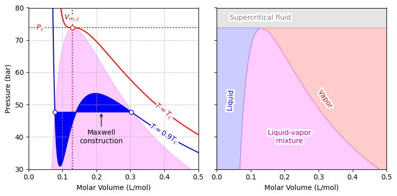

Van der Waals isotherm for CO $_2$ at $T = 0.9\,T_c$ , with the Maxwell construction illustrating how the unphysical loop is replaced by a horizontal tie line defining liquid–vapor coexistence. The critical point at $T = T_c$ is also shown, where the liquid and vapor phases merge.

Expanding Equation (5) and rearranging terms gives a cubic equation for $V_\text{m}$ :

V_\text{m}^3 - \left( b_\text{m} + \frac{R T}{P} \right) V_\text{m}^2 + \frac{a_\text{m}}{P} V_\text{m} - \frac{a_\text{m} b_\text{m}}{P} = 0.

(6)

Complete Derivation of the Cubic Equation in

V_\text{m}

1. Expand Equation (5) and subtract $RT$ from both sides:

P V_\text{m} - P b_\text{m} + \frac{a_\text{m}}{V_\text{m}} - \frac{a_\text{m} b_\text{m}}{V_\text{m}^2} - R T = 0.

(7)

2. Multiply both sides by $V_\text{m}^2 / P$ :

V_\text{m}^3 - b_\text{m} V_\text{m}^2 + \frac{a_\text{m}}{P} V_\text{m} - \frac{a_\text{m} b_\text{m}}{P} - \frac{R T}{P} V_\text{m}^2 = 0.

(8)

3. Group terms:

V_\text{m}^3 - \left( b_\text{m} + \frac{R T}{P} \right) V_\text{m}^2 + \frac{a_\text{m}}{P} V_\text{m} - \frac{a_\text{m} b_\text{m}}{P} = 0.

(9)

At the critical point, the cubic in Equation (6) has a triple root at $V_{\text{m},c}$ , so it can be written as

\left( V_\text{m} - V_{\text{m},c} \right)^3 = V_\text{m}^3 - 3 V_{\text{m},c} V_\text{m}^2 + 3 V_{\text{m},c}^2 V_\text{m} - V_{\text{m},c}^3 = 0.

(10)

Matching coefficients yields

V_{\text{m},c} = 3 b_\text{m}, \quad P_{\text{c}} = \frac{a_\text{m}}{27 b_\text{m}^2}, \quad T_{\text{c}} = \frac{8 a_\text{m}}{27 b_\text{m} R}.

(11)

Complete Derivation of the Critical Point

1. Set coefficients equal and solve for powers of $V_{\text{m},c}$ :

V_{\text{m},c} = \frac{1}{3} \left( b_\text{m} + \frac{R T_{\text{c}}}{P_{\text{c}}} \right), \quad V_{\text{m},c}^2 = \frac{a_\text{m}}{3 P_{\text{c}}}, \quad V_{\text{m},c}^3 = \frac{a_\text{m} b_\text{m}}{P_{\text{c}}}.

(12)

2. Divide $V_{\text{m},c}^3$ by $V_{\text{m},c}^2$ to eliminate $P_{\text{c}}$ :

\begin{aligned} \frac{V_{\text{m},c}^3}{V_{\text{m},c}^2} &= \frac{a_\text{m} b_\text{m}}{P_{\text{c}}} \cdot \frac{3 P_{\text{c}}}{a_\text{m}} \\ V_{\text{m},c} &= 3 b_\text{m}. \end{aligned}

(13)

3. Substitute into $V_{\text{m},c}^3$ and solve for $P_{\text{c}}$ :

\begin{aligned} V_{\text{m},c}^3 &= \frac{a_\text{m} b_\text{m}}{P_{\text{c}}} \\ 27 b_\text{m}^3 &= \frac{a_\text{m} b_\text{m}}{P_{\text{c}}} \\ P_{\text{c}} &= \frac{a_\text{m}}{27 b_\text{m}^2}. \end{aligned}

(14)

4. Substitute these results into $V_{\text{m},c}$ and solve for $T_{\text{c}}$ :

\begin{aligned} V_{\text{m},c} &= \frac{1}{3} \left( b_\text{m} + \frac{R T_{\text{c}}}{P_{\text{c}}} \right) \\ 3 b_\text{m} &= \frac{1}{3} \left( b_\text{m} + R T_{\text{c}} \cdot \frac{27 b_\text{m}^2}{a_\text{m}} \right) \\ 9 b_\text{m} &= b_\text{m} + R T_{\text{c}} \cdot \frac{27 b_\text{m}^2}{a_\text{m}} \\ 8 b_\text{m} &= R T_{\text{c}} \cdot \frac{27 b_\text{m}^2}{a_\text{m}} \\ T_{\text{c}} &= \frac{8 a_\text{m}}{27 b_\text{m} R}. \end{aligned}

(15)

Corresponding States¶

import numpy as np
import pandas as pd
import matplotlib.pyplot as plt
from matplotlib.lines import Line2D
from labellines import labelLines
from scipy.constants import R
from myst_nb import glue

# Define styles for species
style_for_species = {"Ar": 'o', "O2": '^', "H2O": 's', "CO2": 'p'}
label_for_species = {"Ar": "Ar", "O2": "O$_2$", "H2O": "H$_2$O", "CO2": "CO$_2$"}
line_style_for_species = {"Ar": "-", "O2": "--", "H2O": "-.", "CO2": ":"}
color_for_temperature = {0.9: "blue", 1.0: "blue", 1.1: "red", 1.2: "magenta", 2.0: "red"}
color_for_species = {"Ar": "black", "O2": "blue", "H2O": "red", "CO2": "magenta"}

# Paths to data files
paths = [
    f"../_static/section-04/isothermal-properties-for-{species}-Tr={T_r}.csv"
    for species in ["argon", "oxygen", "water", "carbon-dioxide"]
    for T_r in [1.0, 1.2, 2.0]
]

# Create figure
fig, ax = plt.subplots(figsize=(4, 4))

# Load and plot data
for i, path in enumerate(paths):
    df = pd.read_csv(path)
    df.rename(columns={"Temperature (K)": "T", "Pressure (bar)": "P_bar", "Volume (m3/mol)": "Vm"}, inplace=True)
    df["P"] = df["P_bar"] * 1e5  # Convert bar to Pa
    df["Z"] = df["P"] * df["Vm"] / (R * df["T"])
    
    species = df["substance"].values[0]
    T_r = df["Tr"].values[0].round(1)
    color = color_for_temperature[T_r]
    linestyle = line_style_for_species[species]
    label = f"$T_r = {T_r}$" if i % 4 == 0 else None
    
    line = ax.plot(df["Pr"], df["Z"], color=color, linestyle=linestyle, alpha=0.5, label=label)
    if label:
        labelLines(line, align=False, xvals=[2], zorder=2.5)

# Create legend
legend_elements = [Line2D([0], [0], c='k', label=label_for_species[s], ls=line_style_for_species[s], alpha=0.5) 
                   for s in line_style_for_species]
ax.legend(handles=legend_elements, loc='lower right')

# Set labels and grid
ax.set_xlim(0, 8)
ax.set_ylim(0, 1.25)
ax.set_xlabel("Reduced Pressure ($P_r = P / P_c$)")
ax.set_ylabel("$Z$")
ax.grid(True, linestyle="--", alpha=0.7)

plt.tight_layout()
plt.show()
plt.close(fig)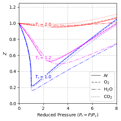

Compressibility factor $Z$ for argon, oxygen, water, and carbon dioxide plotted over a range of reduced pressures for different reduced temperatures. These data illustrate how real gases exhibit similar trends when expressed in terms of their critical properties, consistent with the principle of corresponding states.

Introduce reduced variables $V_{\text{m},r}$ , $P_r$ , and $T_r$ via

V_\text{m} = V_{\text{m},r} V_{\text{m},c}, \quad P = P_r P_c, \quad T = T_r T_c,

(16)

and substitute into Equation (5) to obtain

\left( P_r + \frac{3}{V_{\text{m},r}^2} \right) \left( V_{\text{m},r} - \frac{1}{3} \right) = \frac{8}{3} T_r.

(17)

This corresponding-states form shows that all van der Waals fluids obey the same reduced EOS when expressed relative to their critical properties.

Complete Derivation of the Corresponding States Equation

1. Substitute the reduced-variable definitions into Equation (5):

\left( P_r P_c + \frac{a_\text{m}}{V_{\text{m},r}^2 V_{\text{m},c}^2} \right) \left( V_{\text{m},r} V_{\text{m},c} - b_\text{m} \right) = R T_r T_c.

(18)

2. Divide both sides by $P_c V_{\text{m},c}$ :

\left( P_r + \frac{a_\text{m}}{V_{\text{m},r}^2 V_{\text{m},c}^2 P_c} \right) \left( V_{\text{m},r} - \frac{b_\text{m}}{V_{\text{m},c}} \right) = \frac{R T_c}{P_c V_{\text{m},c}} T_r.

(19)

3. Substitute $P_c$ , $V_{\text{m},c}$ , and $T_c$ in terms of $a_\text{m}$ , $b_\text{m}$ , and $R$ :

\begin{aligned} \left( P_r + \frac{a_\text{m}}{V_{\text{m},r}^2} \cdot \frac{1}{9 b_\text{m}^2} \cdot \frac{27 b_\text{m}^2}{a_\text{m}} \right) \left( V_{\text{m},r} - \frac{b_\text{m}}{3 b_\text{m}} \right) &= R \cdot \frac{8 a_\text{m}}{27 b_\text{m} R} \cdot \frac{27 b_\text{m}^2}{a_\text{m}} \cdot \frac{1}{3 b_\text{m}} T_r \\ \left( P_r + \frac{3}{V_{\text{m},r}^2} \right) \left( V_{\text{m},r} - \frac{1}{3} \right) &= \frac{8}{3} T_r. \end{aligned}

(20)

Computational Studio: Real Gas¶

Explore deviations from ideal behavior by dynamically comparing the ideal-gas, van der Waals (vdW), and Peng–Robinson (PR) equations of state. Adjust temperature and pressure to visualize how intermolecular forces impact the compressibility factor ( $Z$ ) and $P$ – $V_\text{m}$ isotherms, particularly near the critical point.

You can open the studio in a new tab: Real Gas Computational Studio.

Worked Example¶

van der Waals critical constants and $Z_c$ for CO $_2$ ¶

Use the van der Waals parameters used in the section plots: $a_m = 3.6551\ \mathrm{L^2\,bar\,mol^{-2}}$ , $b_m=0.042816\ \mathrm{L\,mol^{-1}}$ , and $R=0.08314\ \mathrm{L\,bar\,mol^{-1}\,K^{-1}}$ .

The van der Waals critical constants are

V_{\mathrm m,c}=3b_m,\qquad P_c=\frac{a_m}{27b_m^2},\qquad T_c=\frac{8a_m}{27b_mR}.

(21)

Critical volume
$V_{\mathrm m,c}=3(0.042816)=0.128448\ \mathrm{L/mol}.$
(22)
Critical pressure
$P_c=\frac{3.6551}{27(0.042816)^2}=73.85\ \mathrm{bar}.$
(23)
Critical temperature
$T_c=\frac{8(3.6551)}{27(0.042816)(0.08314)}=304.2\ \mathrm{K}.$
(24)
Critical compressibility factor
$Z_c \equiv \frac{P_cV_{\mathrm m,c}}{RT_c} =\frac{73.85\times 0.12845}{0.08314\times 304.2} =0.375=\frac{3}{8}.$
(25)

Result. The van der Waals model predicts $T_c\approx 304\ \mathrm{K}$ , $P_c\approx 74\ \mathrm{bar}$ , $V_{\mathrm m,c}\approx 0.128\ \mathrm{L/mol}$ , and $Z_c=3/8$ .

Concept Checks¶

Why can a gas be “coincidentally ideal” (i.e., $Z=1$ ) even when interactions are not negligible?
What physical effects are represented by the $a/V_{\mathrm m}^2$ and $b$ corrections in the van der Waals EOS?
At fixed $T$ , how does $Z$ typically change as $P$ increases, and why?
Why does the reduced-variable form imply similar behavior across different substances at corresponding reduced conditions?

Key Takeaways¶

Nonideality is quantified by $Z=PV/(nRT)$ ; $Z<1$ suggests net attractions and $Z>1$ suggests net repulsions.
The van der Waals EOS introduces an attraction parameter $a$ and an excluded-volume parameter $b$ .
Critical constants follow directly from the cubic form of the van der Waals EOS, with $Z_c=3/8$ .
Using reduced variables $(T_r,P_r,V_r)$ yields the corresponding-states form shared by all van der Waals fluids.

Overview and Learning Objectives¶

Core Ideas and Derivations¶

Deviations from Ideal Behavior¶

Compressibility Factor¶

Van der Waals Fluid¶

Van der Waals Equation of State¶

Van der Waals Isotherm¶

Critical Point¶

Corresponding States¶

Computational Studio: Real Gas¶

Worked Example¶

van der Waals critical constants and ZcZ_cZc​ for CO2_22​¶

Concept Checks¶

Key Takeaways¶

van der Waals critical constants and $Z_c$ for CO $_2$ ¶