2.1. Introduction to Statistical Mechanics

Course-wide Conventions & Notation

Overview and Learning Objectives¶

Statistical mechanics bridges microscopic states and macroscopic thermodynamics by treating measurable quantities as ensemble averages. This section introduces expected values, defines the common ensembles (microcanonical, canonical, and grand canonical), and states the fundamental postulate for an isolated system.

Learning objectives:

• Distinguish an arithmetic average (sample mean) from an ensemble (expected) average $\langle X\rangle$.

• Define microstates, macrostates, and an ensemble, and identify the constraints defining the microcanonical, canonical, and grand canonical ensembles.

• State the fundamental postulate of statistical mechanics for the microcanonical ensemble.

• Compute microcanonical probabilities $p_i=1/M$ and simple expected values from a discrete distribution.

Core Ideas and Derivations¶

Macroscopic Properties as Expected Values of Microscopic Properties¶

A core principle of statistical mechanics is that macroscopic thermodynamic properties are statistical averages (expected values) of microscopic properties.

Arithmetic Average vs. Expected Value¶

In basic statistics, the arithmetic average (sample mean) $\bar{X}$ of a dataset $X=\{X_1, X_2, \ldots, X_M\}$ is:

In statistical mechanics, we typically work with an expected value, which weights each outcome by its probability. For a discrete random variable $X$ that takes values $\{X_i\}$ with probabilities $\{p_i\}$, the expected value is

where $p_i$ is the probability of the $i$-th outcome (microstate), and the sum runs over the microstates included in the ensemble.

In thermodynamics, typical choices of $X$ include the internal energy, enthalpy, or other measurable properties. We will compute such quantities by specifying the probabilities $\{p_i\}$ appropriate to the ensemble of interest.

Ensembles of Microstates¶

Probability of a Microstate in the Microcanonical Ensemble¶

For an isolated system—one that exchanges neither energy nor matter with its surroundings—the appropriate statistical description is the microcanonical ensemble.

Source

import matplotlib.pyplot as plt
import matplotlib.patches as mpatches
from myst_nb import glue

# Helper function to plot a system
def plot_system(ax, title, annotations, boundary_color='b'):
    box = mpatches.FancyBboxPatch((0, 0), 1, 1, boxstyle='roundtooth', ec=boundary_color, fc='w')
    ax.add_patch(box)
    ax.set_title(title, fontsize=14)
    ax.text(0.5, 0.5, 'System', ha='center', va='center', fontsize=12)
    ax.text(0.5, -0.65, 'Surroundings', ha='center', va='center', fontsize=12)
    ax.text(0.5, 1.3, 'Boundary', ha='center', va='bottom', fontsize=12, color=boundary_color)
    for annotation in annotations:
        if "arrowprops" in annotation:  # Arrow annotations
            ax.annotate('', **annotation)
        else:  # Text annotations
            ax.text(**annotation)
    ax.set_xlim(-1, 2)
    ax.set_ylim(-1, 2)
    ax.set_aspect('equal')
    ax.axis('off')

fig, ax = plt.subplots(1, 1, figsize=(4, 4))
plot_system(ax, "", [])

plt.show()
plt.close(fig)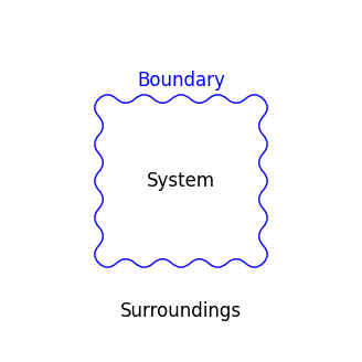

An isolated system exchanges neither energy nor matter with its surroundings.

Fundamental Postulate of Statistical Mechanics¶

Therefore, the probability of finding the system in the $i$-th microstate is

where $M$ is the total number of accessible microstates compatible with $\left(N, V, E\right)$.

Worked Example¶

Expected value vs. arithmetic mean (die rolls)¶

A fair die is rolled $n=300$ times. Let $X_j=1$ if the $j$-th outcome is a six and $X_j=0$ otherwise.

1. One roll

   $$\langle X_j\rangle = 1\cdot \frac{1}{6} + 0\cdot \frac{5}{6} = \frac{1}{6}.$$

   (9)

2. Linearity of expectation

   For independent, identical trials, the expected total number of sixes is the sum of the individual expectations:

   $$\langle N_{\text{sixes}}\rangle = \sum_{j=1}^{300}\langle X_j\rangle = 300\left(\frac{1}{6}\right)=50.$$

   (10)

Result. The expected number of sixes in 300 rolls is 50.

Concept Checks¶

1. In what sense is “temperature” absent from the microcanonical ensemble description?

2. Why is the expected value $\langle X\rangle$ more informative than the arithmetic mean of a single dataset when predicting thermodynamic properties?

3. What physical meaning does “accessible microstate” carry in the fundamental postulate?

4. How would you modify the probability assignment if only a subset of the nominal $M$ microstates were accessible?

Key Takeaways¶

• Macroscopic properties are computed as expected values over microstates.

• An ensemble is a probability model for microstates consistent with specified macroscopic constraints.

• In the microcanonical ensemble, each accessible microstate has equal probability: $p_i=1/M$.

• Choosing the right ensemble is choosing the right constraints: $(N,V,E)$, $(N,V,T)$, or $(\mu,V,T)$.