2.2. Canonical Ensemble

Overview and Learning Objectives¶

The canonical ensemble describes a closed system in thermal contact with a large heat bath at fixed temperature. Its central result is the Boltzmann assignment $p_i \propto e^{-\beta E_i}$ , normalized by the partition function. This section derives and interprets that probability distribution and introduces a two-state system as a concrete model.

In a closed system (energy exchange allowed, matter exchange forbidden) in thermal contact with a heat bath, the appropriate statistical description is the canonical ensemble.

import matplotlib.pyplot as plt
import matplotlib.patches as mpatches
from myst_nb import glue

# Helper function to plot a system
def plot_system(ax, title, annotations, boundary_color='b'):
    box = mpatches.FancyBboxPatch((0, 0), 1, 1, boxstyle='roundtooth', ec=boundary_color, fc='w')
    ax.add_patch(box)
    ax.set_title(title, fontsize=14)
    ax.text(0.5, 0.5, 'System', ha='center', va='center', fontsize=12)
    ax.text(0.5, -0.65, 'Surroundings', ha='center', va='center', fontsize=12)
    ax.text(0.5, 1.3, 'Boundary', ha='center', va='bottom', fontsize=12, color=boundary_color)
    for annotation in annotations:
        if "arrowprops" in annotation:  # Arrow annotations
            ax.annotate('', **annotation)
        else:  # Text annotations
            ax.text(**annotation)
    ax.set_xlim(-1, 2)
    ax.set_ylim(-1, 2)
    ax.set_aspect('equal')
    ax.axis('off')

# Define annotations for each system
annotations = [
        dict(xy=(-0.6, 0.15), xytext=(0.15, 0.15), arrowprops=dict(arrowstyle='<->', color='r')),
        dict(x=-1, y=0.3, s='Energy', ha='left', va='bottom', fontsize=12, color='r'),
]

fig, ax = plt.subplots(1, 1, figsize=(4, 4))
plot_system(ax, "", annotations)

plt.show()
plt.close(fig)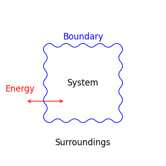

A closed system exchanges energy—but not matter—with its surroundings.

Learning objectives:

Describe the physical meaning of a heat bath and why its temperature is approximately constant during energy exchange.
Derive the canonical probability $p_i = e^{-\beta E_i}/Q$ and define $\beta$ and $Q$ .
Use the partition function $Q=\sum_i e^{-\beta E_i}$ to normalize probabilities and compute ratios $p_j/p_i$ .
Apply the canonical distribution to a two-state system and interpret the low- and high-temperature limits.

Core Ideas and Derivations¶

Probability of a Microstate in the Canonical Ensemble¶

Consider an ensemble of $\mathcal{A}$ identical closed systems in thermal contact with a heat bath at temperature $T$ . A heat bath is an environment so large that it can absorb or release energy with negligible change in temperature.

How Can an Environment Absorb or Release Energy Without Changing Its Temperature?

The key point is that the temperature of a collection of particles is determined by the average kinetic energy per particle. According to the equipartition theorem, for particles with three translational degrees of freedom, the total kinetic energy is

E_{\text{kin}} = \frac{3}{2} N\, k_\text{B}\, T.

(1)

Thus, for a fixed amount of energy transfer, the corresponding change in temperature is

\Delta T = \frac{2}{3}\frac{\Delta E_\text{kin}}{N\, k_\text{B}}.

(2)

Because the environment has many more particles than the system ( $N_\text{env} \gg N_\text{sys}$ ), the same energy transfer $\Delta E$ produces a much smaller $\Delta T$ in the environment. For example, if $N_\text{env} = 10N_\text{sys}$ (e.g., $N_\text{sys} = 6.022\times10^{23}$ and $N_\text{env} = 6.022\times10^{24}$ particles), then the same $\Delta E$ yields a temperature change that is ten times smaller for the environment.

This illustrates why an environment (a heat bath) can absorb or release energy nearly isothermally: its very large number of particles (and hence high heat capacity) makes the fractional change in average kinetic energy per particle negligible, even while energy is exchanged.

Thus, even though the total kinetic energy of the universe (system plus environment) remains constant, the environment’s temperature barely changes because any energy loss or gain is diluted among a huge number of particles.

Population ratios depend only on energy differences¶

Intuition tells us that a system is more likely to be found in lower-energy microstates.

Building This Intuition

Consider a raindrop that can exist at two different elevations: one high up at Lake Itasca in northern Minnesota and one low down in the Mississippi River in St. Louis. At the higher elevation, the raindrop has more gravitational potential energy, making that state less favorable. Consequently, the raindrop is more likely to be found at the lower elevation, where its gravitational potential energy is reduced. In essence, systems tend to prefer lower-energy states, which is why, on a macroscopic scale, water naturally flows downhill.

Let $a_1$ and $a_2$ denote the numbers of systems in microstates 1 and 2. We assume the population ratio depends only on the energy difference:

\frac{a_2}{a_1} = f \left( E_1, E_2 \right) = f \left( E_1 - E_2 \right),

(3)

where $E_1$ and $E_2$ are the corresponding microstate energies.

Why Does the Ratio Depend Only on the Energy Difference?

The energy of a system is defined relative to an arbitrary (often convenient) reference level. For example,

The kinetic energy of a moving particle is defined relative to a stationary particle.
The gravitational potential energy of a raindrop is defined relative to the surface of the Earth.

Therefore, only energy differences—not the absolute zero of energy—enter into probability ratios.

Finding an Acceptable Form for $f$ ¶

Because ratios multiply, we can write

\begin{align*} \frac{a_3}{a_1} &= \frac{a_2}{a_1}\,\frac{a_3}{a_2} \\ f \left( E_1 - E_3 \right) &= f \left( E_1 - E_2 \right)\, f \left( E_2 - E_3 \right). \end{align*}

(4)

If $f$ is well behaved (e.g., continuous, measurable), it must be of the form

f \left( E_m - E_n \right) = e^{\beta \left( E_m - E_n \right)},

(5)

where $\beta$ is an undetermined constant. We will later identify $\beta = \frac{1}{k_\text{B} T}$ .

Checking the Form of

f

Using this form for $f$ , the functional equation is satisfied:

\begin{align*} f(E_1-E_2)\,f(E_2-E_3) &= e^{\beta(E_1-E_2)}\,e^{\beta(E_2-E_3)} \\ &= e^{\beta(E_1-E_3)} \\ &= f(E_1-E_3). \end{align*}

(6)

Converting $f$ to a Probability¶

Separating the indices $m$ and $n$ ,

a_m e^{\beta E_m} = a_n e^{\beta E_n} = \mathcal{C},

(7)

where $\mathcal{C}$ is a constant. Therefore, the number of systems in a microstate with energy $E_m$ is

a_m = \mathcal{C} e^{-\beta E_m}.

(8)

The constant $\mathcal{C}$ is determined by the normalization condition

\sum_m a_m = \mathcal{A} = \mathcal{C} \sum_m e^{-\beta E_m}.

(9)

Solving for $\mathcal{C}$ and substituting into the expression for $a_m$ gives

p_m = \frac{a_m}{\mathcal{A}} = \frac{e^{-\beta E_m}}{\sum_m e^{-\beta E_m}} = \frac{e^{-\beta E_m}}{Q},

(10)

where $p_m$ is the probability of finding the system in microstate $m$ and $Q$ is the partition function.

Alternative derivation roadmap: where does

p_i \propto e^{-\beta E_i}

come from?

We will use the canonical-ensemble probability

p_i \propto e^{-\beta E_i} \quad\text{with}\quad \beta = \frac{1}{k_\text{B} T}

(11)

throughout this module. Before we use it heavily, here are two quick (complementary) ways to see why the exponential “Boltzmann factor” appears.

Setup (common to both routes)¶

System $S$ : a closed system (fixed $N,V$ ) with discrete microstates $i=1,2,\dots$ and energies $E_i$ .
Reservoir / heat bath $R$ : very large, can exchange energy with $S$ , and stays at (approximately) constant temperature $T$ .
Universe $S+R$ is isolated, so the total energy is fixed:
$E_{\text{tot}} = E_i + E_R.$
(12)
Weak coupling: the interaction energy is negligible, so energies add.

The question is: What is the probability $p_i$ that the system is in microstate $i$ ?

Route A: “Counting” argument (microcanonical $\rightarrow$ canonical)¶

Idea: the system is more likely to be in a microstate $i$ if the reservoir has many compatible microstates when the system has energy $E_i$ .

Fundamental postulate for an isolated system (the universe):
all accessible microstates of $S+R$ at fixed $E_{\text{tot}}$ are equally likely.
If $S$ is in microstate $i$ , then $R$ must have energy
$E_R = E_{\text{tot}} - E_i.$
(13)
The number of compatible universe microstates is therefore the number of reservoir microstates at that energy:
$\Omega_R(E_{\text{tot}}-E_i).$
(14)
So
$p_i \propto \Omega_R(E_{\text{tot}}-E_i).$
(15)
Convert multiplicity to entropy using Boltzmann’s definition:
$S_R(E) = k_\text{B} \ln \Omega_R(E).$
(16)
Taking logs,
$\ln p_i = \text{const} + \ln \Omega_R(E_{\text{tot}}-E_i) = \text{const} + \frac{S_R(E_{\text{tot}}-E_i)}{k_\text{B}}.$
(17)
Reservoir is huge $\Rightarrow$ expand $S_R$ in a Taylor series around $E_{\text{tot}}$ .
Because $E_i$ is “small” compared to the reservoir’s energy scale,
$S_R(E_{\text{tot}}-E_i) \approx S_R(E_{\text{tot}}) - E_i\left(\frac{\partial S_R}{\partial E}\right)_{E_{\text{tot}}} + \frac{E_i^2}{2}\left(\frac{\partial^2 S_R}{\partial E^2}\right)_{E_{\text{tot}}} + \cdots$
(18)
Use the thermodynamic definition of temperature (for the reservoir):
$\left(\frac{\partial S}{\partial E}\right)_{V,N} = \frac{1}{T}.$
(19)
So the linear term becomes $-E_i/T$ .
The quadratic term is typically negligible because the reservoir’s heat capacity is enormous:
$\left(\frac{\partial^2 S}{\partial E^2}\right)_{V,N} = -\frac{1}{T^2 C_V},$
(20)
so the correction looks like $-E_i^2/(2T^2 C_V)$ , which is tiny when $C_V$ is very large.
Keep only the dominant (linear) term:
$S_R(E_{\text{tot}}-E_i) \approx S_R(E_{\text{tot}}) - \frac{E_i}{T}.$
(21)
Exponentiate to get the Boltzmann factor:
$p_i \propto \exp\!\left(\frac{S_R(E_{\text{tot}})}{k_\text{B}}\right)\, \exp\!\left(-\frac{E_i}{k_\text{B} T}\right).$
(22)
The first exponential is just a constant (independent of $i$ ), so the physics is:
$\boxed{p_i \propto e^{-E_i/(k_\text{B} T)} \equiv e^{-\beta E_i}} \quad\text{with}\quad \beta \equiv \frac{1}{k_\text{B} T}.$
(23)
Normalize to turn “ $\propto$ ” into “ $=$ ”. Define the partition function
$Q \equiv \sum_i e^{-\beta E_i},$
(24)
so
$\boxed{p_i = \frac{e^{-\beta E_i}}{Q}}.$
(25)

Route B: “Maximum entropy” argument (Gibbs entropy + constraints)¶

Idea: in equilibrium with a heat bath, the system adopts the probability distribution that maximizes entropy subject to what is fixed.

Start from the Gibbs/Shannon entropy functional for a probability distribution $\{p_i\}$ :
$S[\{p_i\}] = -k_\text{B} \sum_i p_i \ln p_i.$
(26)
Impose the two canonical constraints:
- normalization: $\sum_i p_i = 1$
- fixed mean energy: $\sum_i p_i E_i = U$
Maximize $S$ with Lagrange multipliers $\alpha$ and $\lambda$ :
$\delta\Big[-k_\text{B}\sum_i p_i\ln p_i -\alpha\Big(\sum_i p_i-1\Big) -\lambda\Big(\sum_i p_iE_i-U\Big)\Big]=0.$
(27)
The maximizer satisfies
$p_i = \text{const}\times e^{-(\lambda/k_\text{B})E_i}.$
(28)
Rename $\beta \equiv \lambda/k_\text{B}$ :
$p_i \propto e^{-\beta E_i}.$
(29)
Normalize exactly as before:
$p_i=\frac{e^{-\beta E_i}}{Q}, \qquad Q=\sum_i e^{-\beta E_i}.$
(30)
Identify $\beta$ with temperature by using the thermodynamic identity
$\left(\frac{\partial S}{\partial U}\right)_{V,N}=\frac{1}{T}.$
(31)
For the canonical distribution one can show $dS/dU = k_\text{B}\beta$ , so
$\boxed{\beta=\frac{1}{k_\text{B} T}}.$
(32)

Quick checks / intuition (why this form makes sense)¶

Energy differences matter, not absolute zero:
$\frac{p_j}{p_i}=e^{-\beta(E_j-E_i)}.$
(33)
Shifting all energies by a constant leaves all probability ratios unchanged.
Low $T$ (large $\beta$ ): weights concentrate on the lowest-energy microstates.
High $T$ (small $\beta$ ): many microstates become appreciably populated.
Degeneracy is automatic if we sum over microstates:
if many microstates share the same energy, that energy level is more probable because it appears many times in the sum.

Bottom line: In the canonical ensemble, the exponential appears because the reservoir’s multiplicity grows exponentially with its entropy, and the entropy changes approximately linearly with energy over the small energy exchanges relevant to a large heat bath.

Two-State System¶

Consider a system with two microstates (two “levels”): state 1 with energy $E_1$ and state 2 with energy $E_2$ .

Table 1:Chemical Contexts Where a Two-State Approximation Might be Appropriate

Chemical Context	State 1	State 2
Electronic transitions in atoms or molecules	Ground state	Excited state
Donor–acceptor electron transfer	Reduced state	Oxidized state
Molecular isomerization	Reactant	Product
Defects in solids	Defect-free	Defective
Protein folding	Unfolded	Folded

Partition Function for a Two-State System¶

The partition function $Q_\text{two-state}$ for a two-state system is

\begin{align*} Q_\text{two-state} &= e^{-\beta E_1} + e^{-\beta E_2} \\ &= e^{-\beta E_1} \left( 1 + e^{-\beta \Delta E} \right), \end{align*}

(34)

where $\Delta E = E_2 - E_1$ is the energy difference between the two states.

Probability of Finding the System in State 1¶

The probability of finding the system in state 1 is

p_1 = \frac{e^{-\beta E_1}}{Q_\text{two-state}} = \frac{1}{1 + e^{-\beta \Delta E}} = \frac{1}{1 + e^{-\frac{\Delta E}{k_\text{B} T}}}.

(35)

Probability of Finding the System in State 2¶

The probability of finding the system in state 2 is

p_2 = 1 - p_1.

(36)

Partition Function as the Effective Number of Thermally Accessible Microstates¶

import numpy as np
import matplotlib.pyplot as plt
from scipy.constants import k, eV
from labellines import labelLines
from myst_nb import glue
from matplotlib.patches import Rectangle

k_B = k / eV  # Boltzmann constant in eV/K

# Define the partition function for a two-state system
def partition_function_two_state(E1, E2, T):
    beta = 1 / (k_B * T)
    return np.exp(-beta * E1) + np.exp(-beta * E2)

# Calculate the partition function for a two-state system
E1 = 0
E2 = 0.01  # Energy difference between the two states in eV
T_values = np.linspace(1, 1000, 1000)
Q_values = [partition_function_two_state(E1, E2, T) for T in T_values]

# Calculate the probabilities of finding the system in each state for a two-state system
p1_values = [np.exp(-1 / (k_B * T) * E1) / Q for T, Q in zip(T_values, Q_values)]
p2_values = [np.exp(-1 / (k_B * T) * E2) / Q for T, Q in zip(T_values, Q_values)]

# Plot the partition function and the probabilities of finding the system in each state
fig, axs = plt.subplots(1, 2, figsize=(8, 4))

# Plot the partition function on axs[0]
axs[0].plot(T_values, Q_values, 'k-')
axs[0].set_xlabel('Temperature (K)')
axs[0].set_ylabel('$Q_{\\text{two-state}}$')
axs[0].grid(True)
axs[0].annotate(
    '$\\rightarrow 1$ accessible\nmicrostate', xy=(40, Q_values[0] + 0.01), xytext=(300, 1.1),
    arrowprops=dict(arrowstyle='->', color='b'),
    bbox=dict(boxstyle='round,pad=0.3', fc='w', ec='b'),
    ha='center', va='center', color='b'
)
axs[0].annotate(
    '$\\rightarrow 2$ accessible\nmicrostates', xy=(T_values[-1], Q_values[-1]), xytext=(750, 1.7),
    arrowprops=dict(arrowstyle='->', color='m'),
    bbox=dict(boxstyle='round,pad=0.3', fc='w', ec='m'),
    ha='center', va='center', color='m'
)
axs[0].set_xlim(0, 1000)
axs[0].set_ylim(1, 2)

# Plot the probabilities of finding the system in each state on axs[1]
p1_line, = axs[1].plot(T_values, p1_values, 'b-', label='State 1')
p2_line, = axs[1].plot(T_values, p2_values, 'r-', label='State 2')
labelLines([p1_line, p2_line], zorder=2.5)
axs[1].set_xlabel('Temperature (K)')
axs[1].set_ylabel('Probability')
axs[1].grid(True)
axs[1].set_ylim(0, 1)  # ensure y-axis spans from 0 to 1

# Add tall outlined rectangles around the probabilities at low and high temperatures.
# For T -> 0: highlight T from 1 to 50 K.
# For T = 1000: highlight T from 950 to 1000 K.
rect_low = Rectangle((1, 0), 50 - 1, 1, edgecolor='b', facecolor='b', linestyle='-', alpha=0.2)
rect_high = Rectangle((950, 0), 1000 - 950, 1, edgecolor='m', facecolor='m', linestyle='-', alpha=0.2)
axs[1].add_patch(rect_low)
axs[1].add_patch(rect_high)
axs[1].annotate(
    'Only state 1 is accessed', xy=(50, 0.95), xytext=(100, 0.95),
    arrowprops=dict(arrowstyle='-', color='b'),
    ha='left', va='center', color='b'
)
axs[1].annotate(
    'Both states are accessed', xy=(950, 0.05), xytext=(900, 0.05),
    arrowprops=dict(arrowstyle='-', color='m'),
    ha='right', va='center', color='m'
)

plt.tight_layout()
plt.show()
plt.close(fig)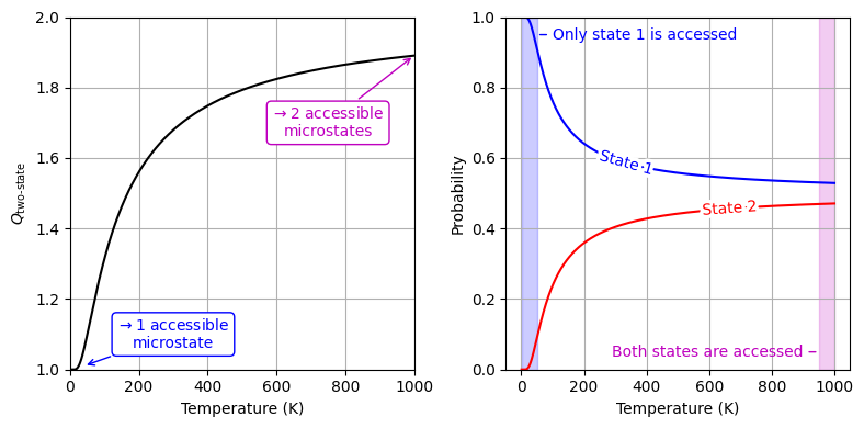

Partition function and state probabilities for a two-state system as a function of temperature ( $\Delta E = 0.01\ \mathrm{eV}$ ).

Computational Studio: Two-State System¶

Explore how the canonical probabilities, partition function, and heat capacity respond to changes in the energy gap and temperature range.

You can open the studio in a new tab: Two-Level System Studio.

Worked Example¶

Two-level system probabilities¶

A single particle has two energy levels: $E_0=0$ and $E_1=\varepsilon$ , with $\varepsilon=0.010\ \mathrm{eV}$ . Find $p_0$ and $p_1$ at $T=300\ \mathrm{K}$ .

Use $p_i = e^{-\beta E_i}/Q$ , $Q=1+e^{-\beta\varepsilon}$ , and $k_\text{B}=8.617\times 10^{-5}\ \mathrm{eV/K}$ .

Compute $\beta\varepsilon$
$\beta\varepsilon=\frac{\varepsilon}{k_\text{B}T} =\frac{0.010}{(8.617\times10^{-5})(300)}=0.387.$
(37)
Compute the Boltzmann factor
$e^{-\beta\varepsilon}=e^{-0.387}=0.679.$
(38)
Normalize
$Q=1+0.679=1.679, \qquad p_0=\frac{1}{Q}=0.596, \qquad p_1=\frac{0.679}{Q}=0.404.$
(39)

Result. At $300\ \mathrm{K}$ , about $40\%$ of systems occupy the excited state for this energy gap.

Concept Checks¶

Why must the argument of the exponential in $e^{-\beta E}$ be dimensionless?
What happens to $p_1/p_0$ as $T\to 0$ ? As $T\to\infty$ ?
Which part of the canonical derivation relies on the reservoir being much larger than the system?
How does shifting all energies by a constant affect $p_i$ , and why?

Key Takeaways¶

In the canonical ensemble, microstate probabilities follow $p_i=e^{-\beta E_i}/Q$ with $\beta=1/(k_\text{B}T)$ .
The partition function $Q$ normalizes probabilities and encodes thermodynamic information.
Probability ratios depend only on energy differences, not on the absolute zero of energy.
Two-level systems vividly illustrate how temperature controls population of higher-energy states.