2.3. Ensemble Averages

Course-wide Conventions & Notation

Overview and Learning Objectives¶

Once microstate probabilities are known, thermodynamic properties follow as ensemble averages. This section derives canonical expressions for internal energy, heat capacity, and pressure in terms of derivatives of $\ln Q$. A recurring theme is that fluctuations are not a nuisance—they encode response functions such as $C_V$.

Section 2.1 emphasized that macroscopic properties are expectation values of microscopic properties, with the expectation taken over the microstate probabilities. Section 2.2 derived the canonical probability distribution for a closed system’s microstates. Here, we connect these results by computing ensemble averages that determine macroscopic properties.

Learning objectives:

• Compute internal energy both as an ensemble average, $U=\langle E\rangle$, and as a derivative, $U=-(\partial\ln Q/\partial\beta)_{N,V}$.

• Relate heat capacity to energy fluctuations via $\sigma_E^2 = k_{\mathrm B}T^2 C_V$.

• Compute pressure from the partition function using $P=k_{\mathrm B}T(\partial\ln Q/\partial V)_{N,T}$ (when applicable).

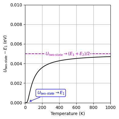
• Apply these formulas to simple discrete models (e.g., a two-state system).

Core Ideas and Derivations¶

Thermodynamic Equilibrium¶

Recall from Section 1.1 that thermodynamic equilibrium is a state of simultaneous mechanical, thermal, and chemical equilibrium. Below are working definitions of each type of equilibrium:

Internal Energy¶

The internal energy $U$ of a macroscopic system at thermodynamic equilibrium is defined as the ensemble average $\langle E \rangle$ of the microstate energy $E$:

where $E_i$ is the energy of microstate $i$, $p_i$ is the probability of that microstate, and $M$ is the total number of microstates.

For the canonical ensemble, using the Boltzmann factor and the partition function $Q$, we have

where $\beta = 1/(k_{\mathrm B} T)$ and

Partial Derivative of the Partition Function¶

Taking the partial derivative of $Q$ with respect to $\beta$ gives

Substituting this result into the expression for $U$ yields

Example: Two-State System¶

For a two-state system with energies $E_1$ and $E_2$, the partition function is

Then the internal energy is

which is the ensemble average $\langle E\rangle$.

Source

import numpy as np
import matplotlib.pyplot as plt
from scipy.constants import k, eV
from labellines import labelLines

kB = k / eV  # Boltzmann constant in eV/K

# Define the partition function for a two-state system
def partition_function_two_state(E1, E2, T):
    beta = 1 / (kB * T)
    return np.exp(-beta * E1) + np.exp(-beta * E2)

# Calculate the partition function for a two-state system
E1 = 0
E2 = 0.01  # Energy difference between the two states in eV
T_values = np.linspace(1, 1000, 1000)
Q_values = [partition_function_two_state(E1, E2, T) for T in T_values]

# Calculate the internal energy for a two-state system
beta_values = 1 / (kB * T_values)
ln_Q_values = np.log(Q_values)
U_values = -np.gradient(ln_Q_values, beta_values)

# Plot the internal energy as a function of temperature
fig, ax = plt.subplots(figsize=(4, 4))
ax.plot(T_values, U_values, 'k-')
ax.set_xlabel('Temperature (K)')
ax.set_ylabel('$U_{\\text{two-state}} - E_1$ (eV)')
ax.grid(True)
ax.annotate(
    '$U_{\\text{two-state}} \\rightarrow E_1$', xy=(40, U_values[0] + 0.0001), xytext=(300, 0.001),
    arrowprops=dict(arrowstyle='->', color='b'),
    bbox=dict(boxstyle='round,pad=0.3', fc='w', ec='b'),
    ha='center', va='center', color='b'
)
x_values_high_T = np.linspace(0, 1000, 1001)
y_values_high_T = ((E1 + E2) / 2) * np.ones_like(x_values_high_T)
line = ax.plot(x_values_high_T, y_values_high_T, 'm--', label='$U_{\\text{two-state}} \\rightarrow (E_1 + E_2) / 2$')
labelLines(line, zorder=2.5)
ax.set_xlim(0, 1000)
ax.set_ylim(0, 0.01)

plt.tight_layout()
plt.show()
plt.close(fig)

Internal energy of a two-state system as a function of temperature, for an energy gap of $0.01\ \mathrm{eV}$.

Heat Capacity at Constant Volume¶

From Section 1.1, heat is energy transferred due to a temperature difference. The heat capacity at constant volume, $C_V$, measures how much heat is required to change a system’s temperature at fixed $N$ and $V$:

Heat Capacity and Energy Fluctuations¶

In statistics, the variance $\sigma_X^2$ of a random variable $X$ is $\sigma_X^2 = \langle (X - \langle X\rangle)^2\rangle$. In statistical mechanics, $\sigma_E^2$ quantifies fluctuations in the total energy:

One can show that

which implies

Pressure¶

In Module 5, we will derive:

1. $A = -k_{\mathrm B}\,T\ln Q$, where $A$ is the Helmholtz free energy.

2. $P = -\left(\frac{\partial A}{\partial V}\right)_{N,T}$, where $P$ is pressure.

Combining these expressions gives

Worked Example¶

Two-state internal energy and heat capacity¶

Consider a two-state system with $E_1=0$ and $E_2=\varepsilon$. Let $x\equiv \beta\varepsilon$.

1. Partition function

   $$Q=1+e^{-x}.$$

   (19)

2. Internal energy

   $$U=\frac{0\cdot 1+\varepsilon e^{-x}}{1+e^{-x}} =\varepsilon\frac{e^{-x}}{1+e^{-x}}.$$

   (20)

3. Heat capacity at constant volume

   Differentiate $U$ with respect to $T$ (holding $N$ and $V$ fixed). Using $x=\varepsilon/(k_{\mathrm B}T)$ and $dx/dT=-x/T$,

   $$C_V=\left(\frac{\partial U}{\partial T}\right)_{N,V} = k_{\mathrm B}\,x^2\,\frac{e^{-x}}{(1+e^{-x})^2}.$$

   (21)

4. Numerical illustration

   For $\varepsilon=0.010\ \mathrm{eV}$ at $T=300\ \mathrm{K}$, $x=0.387$ and $e^{-x}=0.679$, so

   $$U = 0.010\ \mathrm{eV}\times \frac{0.679}{1.679}=4.04\times 10^{-3}\ \mathrm{eV}, \qquad \frac{C_V}{k_{\mathrm B}}=x^2\frac{0.679}{1.679^2}=3.60\times 10^{-2}.$$

   (22)

Result. $U$ interpolates between 0 and $\varepsilon/2$, while $C_V$ peaks when thermal energy is comparable to $\varepsilon$.

Concept Checks¶

1. Why is $U$ obtained from a derivative of $\ln Q$ rather than from $Q$ directly?

2. What does it mean physically when $C_V$ is large? When it is small?

3. In the two-state model, why does $C_V\to 0$ both as $T\to 0$ and as $T\to\infty$?

4. How do fluctuations in energy relate to the system’s ability to exchange heat with a reservoir?

Key Takeaways¶

• Thermodynamic properties are ensemble averages computed from microstate probabilities.

• In the canonical ensemble, $U=-(\partial\ln Q/\partial\beta)_{N,V}$.

• Response functions connect to fluctuations: $\sigma_E^2=k_{\mathrm B}T^2C_V$.

• Simple discrete models already capture key qualitative behaviors of $U(T)$ and $C_V(T)$.