2.7. Linear Rigid Rotor - Physical Chemistry II

Overview and Learning Objectives¶

The linear rigid rotor models molecular rotation (especially for diatomics) and provides the rotational partition function used in molecular thermodynamics. We derive the quantized rotational levels and their degeneracies, develop the high- $T$ approximation $q_{\mathrm{rot}}\approx T/(\sigma\Theta_{\mathrm{rot}})$ , and obtain the corresponding rotational contributions to the internal energy and heat capacity.

Learning objectives:

State the rigid-rotor energy levels $E_J=\hbar^2J(J+1)/(2I)$ and degeneracy $g_J=2J+1$ .
Write the rotational partition function as a sum over $J$ , including degeneracy.
Derive the high- $T$ approximation and define the rotational temperature $\Theta_{\mathrm{rot}}=\hbar^2/(2k_{\mathrm{B}}I)$ .
Compute rotational contributions to $U$ and $C_V$ in the classical limit, and interpret the symmetry factor $\sigma$ .

Core Ideas and Derivations¶

Review of the Linear Rigid Rotor¶

import numpy as np
import matplotlib.pyplot as plt
from mpl_toolkits.mplot3d.art3d import Poly3DCollection
from scipy.constants import k, eV
from labellines import labelLines
from myst_nb import glue

fig, axs = plt.subplot_mosaic([[0]], figsize=(4, 4))

# Plot the energy levels (blue lines)
for J in range(0, 3):
    g_J = 2 * J + 1
    x_min = -0.04 - 0.1 * (g_J - 1) / 2
    for i in range(g_J):
        # Plot each degenerate sub-level horizontally
        if i == (g_J - 1) / 2:
            energy_line = axs[0].plot(
                [x_min, x_min + 0.08], 
                [J * (J + 1), J * (J + 1)], 
                color='blue',
                label=r'$E_{%d}$' % J
            )
        else:
            axs[0].plot(
                [x_min, x_min + 0.08], 
                [J * (J + 1), J * (J + 1)], 
                color='blue'
            )
        x_min += 0.1
    # Label only one line at each J for clarity
    labelLines(energy_line, zorder=2.5)

axs[0].set_ylabel('Energy (arb. units)')
axs[0].set_xticks([])
axs[0].set_yticks([])
axs[0].spines['top'].set_visible(False)
axs[0].spines['bottom'].set_visible(False)
axs[0].spines['right'].set_visible(False)
axs[0].spines['left'].set_visible(False)

plt.tight_layout()
plt.show()
plt.close(fig)

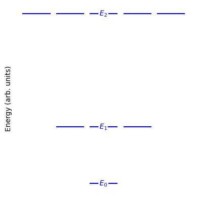
Energy levels for a linear rigid rotor. Each level $E_J$ has degeneracy $g_J = 2J + 1$ (magnetic quantum numbers $m=-J,\ldots,J$ ). For example, the $J=2$ level contains five degenerate microstates with $m=-2,-1,0,1,2$ .

For a linear rigid rotor with moment of inertia $I$ , the energy levels are:

E_J \;=\; \frac{\hbar^2}{2I}\,J\bigl(J+1\bigr) \quad\text{for}\quad J = 0, 1, 2, \dots

(1)

Here, $\hbar$ is the reduced Planck constant, and $g_J=2J+1$ is the degeneracy of the level $E_J$ .

Partition Function for a Linear Rigid Rotor¶

In the canonical ensemble, the rotational partition function is

q_{\mathrm{rot}} \;=\; \sum_{i=0}^\infty e^{-\beta E_i} \;=\; \sum_{J=0}^\infty g_J \, e^{-\beta\,E_J} \;=\; \sum_{J=0}^\infty (2J+1)\,\exp\!\Bigl[-\beta \,\frac{\hbar^2}{2I}\,J(J+1)\Bigr].

(3)

Summation vs. Levels

Sum over $i$ : sums over individual microstates (each degenerate sub-level).
Sum over $J$ : reorganizes the sum by energy level $E_J$ , factoring in the degeneracy $g_J = 2J+1$ .

High-Temperature Approximation¶

When $k_{\mathrm{B}}T \gg \frac{\hbar^2}{2I}$ , we can approximate the discrete sum by treating $J$ as continuous and converting the sum to an integral. Define

x \;=\; J(J+1), \quad dx \;=\; (2J+1)\,dJ.

(4)

Then

q_{\mathrm{rot}} \;\approx\; \int_{0}^{\infty} (2J+1)\,\exp\Bigl[-\beta \,\frac{\hbar^2}{2I}\,J(J+1)\Bigr]\;dJ \;=\; \int_{x=0}^{\infty} \exp\Bigl[-\beta \,\tfrac{\hbar^2}{2I}\,x\Bigr]\;dx.

(5)

Evaluating the integral gives

\int_{0}^{\infty} \exp\Bigl[-\beta \,\tfrac{\hbar^2}{2I}\,x\Bigr]\;dx \;=\; \frac{1}{\beta \,\frac{\hbar^2}{2I}} \;=\; \frac{2I\,k_{\mathrm{B}} T}{\hbar^2}.

(6)

We define the rotational temperature $\Theta_{\mathrm{rot}}$ by

\Theta_{\mathrm{rot}} \;=\; \frac{\hbar^2}{2k_{\mathrm{B}}\,I}.

(7)

Thus, for a heteronuclear diatomic rotor (symmetry factor $\sigma=1$ ),

q_{\mathrm{rot}} \;\approx\; \frac{2I\,k_{\mathrm{B}} T}{\hbar^2} \;=\; \frac{T}{\Theta_{\mathrm{rot}}}.

(8)

Ensemble Averages¶

Natural Logarithm of the Partition Function¶

From the high- $T$ approximation (with $\sigma=1$ for simplicity),

\ln q_{\mathrm{rot}} \;=\; \ln \Bigl(\tfrac{T}{\Theta_{\mathrm{rot}}}\Bigr) \;=\; \ln T \;-\;\ln \Theta_{\mathrm{rot}}.

(10)

Internal Energy¶

The rotational internal energy (per rotor) is

U_{\mathrm{rot}} \;=\; - \left(\frac{\partial \ln q_{\mathrm{rot}}}{\partial \beta}\right)_{N,V} \;=\; k_{\mathrm{B}}\,T^2 \left(\frac{\partial \ln q_{\mathrm{rot}}}{\partial T}\right)_{N,V}.

(11)

Since $\ln q_{\mathrm{rot}}=\ln T-\ln \Theta_{\mathrm{rot}}$ , we have

\frac{\partial \ln q_{\mathrm{rot}}}{\partial T} \;=\; \frac{\partial}{\partial T}\bigl(\ln T\bigr) \;=\; \frac{1}{T}.

(12)

Hence,

U_{\mathrm{rot}} \;=\; k_{\mathrm{B}} \, T.

(13)

Heat Capacity at Constant Volume¶

The rotational contribution to the heat capacity (per rotor) is

C_V^{(\mathrm{rot})} \;=\; \left(\frac{\partial U_{\mathrm{rot}}}{\partial T}\right)_{N,V} \;=\; k_{\mathrm{B}}.

(14)

Physically, this means a single linear rotor contributes $k_{\mathrm{B}}$ to the heat capacity in the classical (high- $T$ ) limit, corresponding to two rotational degrees of freedom (each contributing $\tfrac{1}{2}k_{\mathrm{B}}$ ).

Computational Studio: Linear Rigid Rotor¶

Explore how molecular geometry and symmetry impact rotational thermodynamics. Use this studio to visualize the rotor, analyze the population distribution across quantum states, and compare the partition function and entropy of heteronuclear vs. homonuclear diatomic molecules.

You can open the studio in a new tab: Rigid Rotor Computational Studio.

Worked Example¶

Rotational temperature and $q_{\mathrm{rot}}$ for CO

Approximate CO as a rigid rotor with bond length $r = 1.128\ \text{\AA} = 1.128\times10^{-10}\ \mathrm{m}$ . Use $m_C=12u$ , $m_O=16u$ , and $u=1.66054\times10^{-27}\ \mathrm{kg}$ .

Reduced mass
$\mu=\frac{m_Cm_O}{m_C+m_O} =\frac{(12u)(16u)}{28u}=6.857u =1.14\times10^{-26}\ \mathrm{kg}.$
(15)
Moment of inertia
$I=\mu r^2=(1.14\times10^{-26})(1.128\times10^{-10})^2 =1.45\times10^{-46}\ \mathrm{kg\,m^2}.$
(16)
Rotational temperature
$\Theta_{\mathrm{rot}}=\frac{\hbar^2}{2k_{\mathrm{B}}I} =\frac{(1.055\times10^{-34})^2}{2(1.381\times10^{-23})(1.45\times10^{-46})} \approx 2.78\ \mathrm{K}.$
(17)
High- $T$ partition function (heteronuclear, $\sigma=1$ ) at $T=300\ \mathrm{K}$
$q_{\mathrm{rot}}\approx \frac{T}{\Theta_{\mathrm{rot}}}=\frac{300}{2.78}\approx 1.08\times10^{2}.$
(18)

Result. For CO at room temperature, $T\gg \Theta_{\mathrm{rot}}$ , so the high- $T$ approximation is well justified.

Concept Checks¶

Why does each $J$ level have degeneracy $2J+1$ ? What symmetry is responsible?
What changes in the partition function when the molecule is homonuclear rather than heteronuclear?
Why does the classical (high- $T$ ) rotor have $U_{\mathrm{rot}}=k_{\mathrm{B}}T$ per molecule?
What physical parameter(s) of the molecule increase $\Theta_{\mathrm{rot}}$ ?

Key Takeaways¶

Rigid-rotor levels scale as $J(J+1)$ with degeneracy $2J+1$ .
In the high- $T$ limit, $q_{\mathrm{rot}}\approx T/(\sigma\Theta_{\mathrm{rot}})$ .
$\Theta_{\mathrm{rot}}$ is set by the moment of inertia $I=\mu r^2$ ; small, stiff molecules have larger $\Theta_{\mathrm{rot}}$ .
Rotational contributions approach equipartition values at sufficiently high temperature.