2.6. Harmonic Oscillator - Physical Chemistry II

Overview and Learning Objectives¶

The quantum harmonic oscillator is a canonical model for molecular vibrations and lattice modes in solids. In this section we derive the oscillator partition function, compute ensemble averages such as internal energy and heat capacity, and examine how the classical (equipartition) limit emerges when $T\gg \Theta_{\mathrm{vib}}$ . We begin with a review of the one-dimensional oscillator, then connect the result to three-dimensional oscillators in the Einstein model.

Learning objectives:

State the harmonic oscillator energy levels $E_n=\hbar\omega(n+\tfrac12)$ and write the corresponding partition function
Evaluate the geometric series to obtain $q = e^{-\beta\hbar\omega/2}/(1-e^{-\beta\hbar\omega})$
Derive the mean energy $U=\tfrac12\hbar\omega+\hbar\omega/(e^{\beta\hbar\omega}-1)$ and interpret the zero-point energy
Use the vibrational temperature $\Theta_{\mathrm{vib}}=\hbar\omega/k_{\mathrm B}$ to analyze low- and high-temperature limits and connect to the Einstein model

Core Ideas and Derivations¶

Review of the One-Dimensional Harmonic Oscillator¶

import numpy as np
import matplotlib.pyplot as plt
from mpl_toolkits.mplot3d.art3d import Poly3DCollection
from scipy.constants import k, eV
from scipy.special import hermite, factorial
from labellines import labelLines
from myst_nb import glue
from numpy.linalg import eigh

fig, axs = plt.subplot_mosaic([[0]], figsize=(4, 4))

def harmonic_potential(x, m, omega):
    """
    Calculates the potential matrix for a particle in a one-dimensional harmonic potential
    
    Parameters
    ----------
    x : array-like
        The positions of the particles.
    m : float
        The mass of the particle.
    omega : float
        The frequency of the harmonic potential
    
    Returns
    -------
    array
        The potential matrix.
    """
    V = 0.5 * m * omega**2 * x**2
    V_matrix = np.diag(V)
    return V_matrix

def off_diagonal_identity_matrix(n_points):
    matrix = np.zeros((n_points, n_points))
    for i in range(n_points):
        if i == 0:
            matrix[i + 1, i] = 1
        elif i == n_points - 1:
            matrix[i - 1, i] = 1
        else:
            matrix[i - 1, i] = 1
            matrix[i + 1, i] = 1
    return matrix

def laplacian_matrix(x):
    """
    Calculates the Laplacian matrix for a particle in a one-dimensional potential.
    
    Parameters
    ----------
    x : array-like
        The positions of the particles.
    
    Returns
    -------
    array
        The Laplacian matrix.
    """
    Delta_x = x[1] - x[0]
    n_points = len(x)
    off_diag = off_diagonal_identity_matrix(n_points)
    Laplacian = (1 / (Delta_x**2)) * (-2 * np.eye(n_points) + off_diag)
    return Laplacian

# Define constants in atomic units
hbar = 1
m = 1

# Harmonic potential
omega = 1

# Discretize the system
n_points = 2000
L = 40
x = np.linspace(-L/2, L/2, n_points)

# Construct the Hamiltonian matrix
H_harm = -hbar**2 / (2 * m) * laplacian_matrix(x) + harmonic_potential(x, m=1, omega=1)

# Solve for eigenvalues and eigenfunctions
E_harm, psi_harm = np.linalg.eigh(H_harm)

# Plot a one-dimensional quadratic potential
axs[0].plot(x, np.diag(harmonic_potential(x, m, omega)), "k-", zorder=2.5, lw=4)

# Plot the energy levels (blue lines)
for n in range(4):
    energy = axs[0].plot(x, np.ones_like(x) * E_harm[n], color='blue', label=r'$E_{%d}$' % n)
    labelLines(energy, xvals=[-L/24], zorder=2.5)

# Plot the wavefunctions (red curves)
for n in range(4):
    wavefunction = axs[0].plot(x, psi_harm[:, n] * 4 + E_harm[n], color='red', label=r'$\psi_{%d}$' % n)
    labelLines(wavefunction, xvals=[L/24], zorder=2.5)

# Format plot
axs[0].set_xlim(-L/8, L/8)
ymin = np.min(np.diag(harmonic_potential(x, m, omega)))
ymax = np.max(psi_harm[:, -1]) + E_harm[3]
yrange = ymax - ymin
ybuffer = 0.05 * yrange
axs[0].set_ylim(ymin - ybuffer, ymax + ybuffer * 2)
axs[0].set_xlabel("Position")
axs[0].set_ylabel("Energy")
axs[0].set_xticks([])
axs[0].set_yticks([])
axs[0].spines['top'].set_visible(False)
axs[0].spines['right'].set_visible(False)
axs[0].spines['left'].set_visible(False)
axs[0].spines['bottom'].set_visible(False)

plt.tight_layout()
plt.show()
plt.close(fig)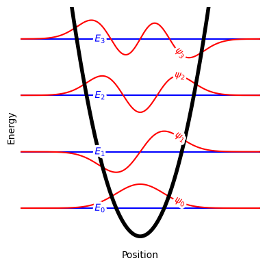

Energy levels and wavefunctions for a one-dimensional harmonic oscillator. The energy levels $E_n$ are shown as blue lines, while the wavefunctions $\psi_n$ are shown as red curves.

For a one-dimensional harmonic oscillator with angular frequency $\omega$ , the quantized energy levels are

E_n = \hbar \omega \left( n + \frac{1}{2} \right) \quad \text{for} \; n = 0, 1, 2, \ldots,

(1)

where $\hbar$ is the reduced Planck constant and $n$ is a nonnegative integer.

Partition Function for a Harmonic Oscillator¶

The (single-oscillator) partition function for a one-dimensional harmonic oscillator is

\begin{aligned} q &= \sum_{n=0}^{\infty} e^{-\beta E_n} \\ &= \sum_{n=0}^{\infty} e^{-\beta \hbar \omega (n + 1/2)} \\ &= e^{-\beta \hbar \omega / 2} \sum_{n=0}^{\infty} e^{-\beta \hbar \omega n}. \end{aligned}

(2)

Evaluation of the Sum¶

The term $\sum_{n=0}^{\infty} e^{-\beta \hbar \omega n}$ is a geometric series. For $|x| < 1$ ,

\sum_{n=0}^{\infty} x^n = \frac{1}{1 - x}.

(3)

Substituting $x = e^{-\beta \hbar \omega}$ gives

q = \frac{e^{-\beta \hbar \omega / 2}}{1 - e^{-\beta \hbar \omega}}.

(4)

Check that

|x| < 1

\begin{aligned} |x| &< 1 \\ \left| e^{-\beta \hbar \omega} \right| &< 1 \\ e^{-\beta \hbar \omega} &< 1 \\ \beta \hbar \omega &> 0 \\ \beta &> 0. \end{aligned}

(5)

Ensemble Averages for a Harmonic Oscillator¶

Natural Logarithm of the Partition Function¶

Taking the natural logarithm of $q$ gives

\ln q = -\frac{\beta \hbar \omega}{2} - \ln(1 - e^{-\beta \hbar \omega}).

(6)

Internal Energy¶

For a single oscillator, the mean energy (internal energy) follows from

U = -\frac{\partial \ln q}{\partial \beta} = \frac{\hbar \omega}{2} + \frac{\hbar \omega}{e^{\beta \hbar \omega} - 1}.

(7)

Derivative of

\ln(1 - e^{-\beta \hbar \omega})

\begin{aligned} \frac{\partial}{\partial \beta} \ln(1 - e^{-\beta \hbar \omega}) &= \frac{1}{1 - e^{-\beta \hbar \omega}} \frac{\partial}{\partial \beta}\left(1 - e^{-\beta \hbar \omega}\right) \\ &= \frac{\hbar \omega\, e^{-\beta \hbar \omega}}{1 - e^{-\beta \hbar \omega}} = \frac{\hbar \omega}{e^{\beta \hbar \omega} - 1}. \end{aligned}

(8)

It is often convenient to define the vibrational temperature $\Theta_{\mathrm{vib}}$ as

\Theta_{\mathrm{vib}} = \frac{\hbar \omega}{k_{\mathrm B}}.

(9)

Using $\beta \hbar \omega = \Theta_{\mathrm{vib}}/T$ , the internal energy can be written as

U = \frac{\hbar \omega}{2} + \frac{\hbar \omega}{e^{\Theta_{\mathrm{vib}} / T} - 1} = k_{\mathrm B}\Theta_{\mathrm{vib}}\left[\frac{1}{2}+\frac{1}{e^{\Theta_{\mathrm{vib}}/T}-1}\right].

(10)

import numpy as np
import matplotlib.pyplot as plt
from mpl_toolkits.mplot3d.art3d import Poly3DCollection
from scipy.constants import k, eV
from labellines import labelLines
from myst_nb import glue

kB = k / eV  # Boltzmann constant in eV/K

fig, axs = plt.subplot_mosaic([[0]], figsize=(4, 4))

Theta_vib = 805  # K, for a Cl2 molecule
hbar_omega = kB * Theta_vib
T = np.linspace(10, 1000, 100)
Tr = T / Theta_vib

U = hbar_omega / 2 + hbar_omega / (np.exp(Theta_vib / T) - 1)

axs[0].plot(Tr, U / hbar_omega, "k-")

axs[0].set_xlabel(r"$T / \Theta_{\text{vib}}$")
axs[0].set_ylabel(r"$U / \left( \hbar \omega \right)$")

zero_point_energy = axs[0].plot([np.min(Tr), np.max(Tr)], [0.5, 0.5], "b--", label="Zero-point energy")
labelLines(zero_point_energy, zorder=2.5)

x = Tr[Tr >= 0.5]
kT = axs[0].plot(x, x, "r--", label=r"$U \rightarrow k_{\text{B}} T$")
labelLines(kT, xvals=[Tr[-1] * 3 / 4], zorder=2.5)

plt.tight_layout()
plt.show()
plt.close(fig)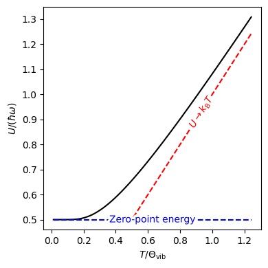

Internal energy of a harmonic oscillator as a function of temperature. The zero-point energy is shown as a blue dashed line, while the high-temperature limit is shown as a red dashed line.

Heat Capacity at Constant Volume¶

In Section 2.3, we showed that

\sigma_E^2 = \left( \frac{\partial^2 \ln q}{\partial \beta^2} \right) = k_{\mathrm B} T^2 C_V.

(11)

From Equation (6), it follows that

C_V = k_{\mathrm B} \left( \frac{\hbar \omega}{k_{\mathrm B} T} \right)^2 \frac{e^{\hbar \omega / k_{\mathrm B} T}}{\left( e^{\hbar \omega / k_{\mathrm B} T} - 1 \right)^2} = k_{\mathrm B} \left( \frac{\Theta_{\mathrm{vib}}}{T} \right)^2 \frac{e^{\Theta_{\mathrm{vib}} / T}}{\left( e^{\Theta_{\mathrm{vib}} / T} - 1 \right)^2}.

(12)

Complete Derivation of

C_V

\begin{aligned} \sigma_E^2 &= \frac{\partial^2}{\partial \beta^2}\left( -\frac{\beta \hbar \omega}{2} - \ln(1 - e^{-\beta \hbar \omega}) \right) \\ &= \frac{\partial}{\partial \beta}\left( -\frac{\hbar \omega}{2} - \frac{\hbar \omega}{e^{\beta \hbar \omega} - 1} \right) \\ &= -\hbar \omega \left( \frac{\partial g^{-1}}{\partial g} \frac{\partial g}{\partial \beta} \right) \quad \text{where} \; g = e^{\beta \hbar \omega} - 1 \\ &= \frac{\hbar \omega}{g^2} \left( \frac{\partial}{\partial \beta} \left( e^{\beta \hbar \omega} - 1 \right) \right) \\ &= \left( \hbar \omega \right)^2 \frac{e^{\beta \hbar \omega}}{\left( e^{\beta \hbar \omega} - 1 \right)^2}. \end{aligned}

(13)

fig, axs = plt.subplot_mosaic([[0]], figsize=(4, 4))

Cv = kB * (Theta_vib / T)**2 * np.exp(Theta_vib / T) / (np.exp(Theta_vib / T) - 1)**2

axs[0].plot(Tr, Cv / kB, "k-")

axs[0].annotate(
    '$C_V \\rightarrow 0$', xy=(0.15, 0), xytext=(Tr[-1] / 3, 0.1),
    arrowprops=dict(arrowstyle='->', color='b'),
    bbox=dict(boxstyle='round,pad=0.3', fc='w', ec='b'),
    ha='center', va='center', color='b'
)

high_T = axs[0].plot([0, Tr[-1]], [1, 1], "r--", label="$C_V \\rightarrow k_{\\text{B}}$")
labelLines(high_T, zorder=2.5)

axs[0].set_xlabel(r"$T / \Theta_{\text{vib}}$")
axs[0].set_ylabel(r"$C_V / k_{\text{B}}$")

plt.tight_layout()
plt.show()
plt.close(fig)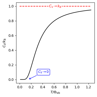

Heat capacity at constant volume of a harmonic oscillator as a function of temperature. The low-temperature limit is indicated by the blue arrow, while the high-temperature limit is shown as a red dashed line.

Computational Studio: Harmonic Oscillator¶

Explore how the internal energy and heat capacity evolve with the characteristic temperature, visualizing the transition between quantum “freeze-out” and the classical high-temperature limit.

You can open the studio in a new tab: Harmonic Oscillator Studio.

Einstein Model¶

The Einstein model is a simple model for an atomic crystal, where $N$ identical atoms occupy lattice sites and vibrate about these sites as independent (i.e., non-interacting) three-dimensional harmonic oscillators, all with the same frequency. Because the atoms occupy fixed lattice sites, they can be treated as distinguishable. For the Einstein model, the partition function is

Q = q^{3N} = \left( \frac{e^{-\beta \hbar \omega / 2}}{1 - e^{-\beta \hbar \omega}} \right)^{3N}.

(14)

One can show that

U = \frac{3}{2} N \hbar \omega + \frac{3N \hbar \omega}{e^{\beta \hbar \omega} - 1},

(15)

and

C_V = 3 N k_{\mathrm B} \left( \frac{\hbar \omega}{k_{\mathrm B} T} \right)^2 \frac{e^{\hbar \omega / k_{\mathrm B} T}}{\left( e^{\hbar \omega / k_{\mathrm B} T} - 1 \right)^2}.

(16)

Dulong–Petit Law¶

# https://en.wikipedia.org/wiki/Heat_capacities_of_the_elements_(data_page)

import pandas as pd

df = pd.read_csv("../_static/chapter-02/section-06/dulong_petit.csv")
df = df[df.Source == "use"].copy()
df["Atomic Number"] = df["Atomic Number"].astype(int)
df["Molar (J/mol·K)"] = df["Molar (J/mol·K)"].astype(float)
df["Molar (R)"] = df["Molar (J/mol·K)"] / 8.314
df["Absolute Deviation"] = np.abs(df["Molar (R)"] - 3)

# Remove elemental gases
elemental_gases = ["H", "He", "N", "O", "F", "Ne", "Cl", "Ar", "Kr", "Xe", "Rn"]
df = df[~df.Symbol.isin(elemental_gases)]

fig, axs = plt.subplot_mosaic([[0]], figsize=(4, 4))

axs[0].scatter(df["Atomic Number"], df["Molar (R)"], color="black")
axs[0].set_xlabel("Atomic Number")
axs[0].set_ylabel(r"Molar heat capacity ($C/R$)")

# Annotate outliers
outliers = df[df["Absolute Deviation"] > 1]
for _, row in outliers.iterrows():
    axs[0].annotate(row["Symbol"], (row["Atomic Number"], row["Molar (R)"]))

# Plot Dulong-Petit law
dulong_petit = axs[0].plot([0, 100], [3, 3], "r--", label="Dulong–Petit law")
labelLines(dulong_petit, zorder=2.5)

plt.tight_layout()
plt.show()
plt.close(fig)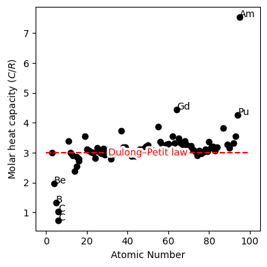

Molar heat capacity of elemental solids as a function of atomic number. The Dulong–Petit law is shown as a red dashed line.

Worked Example¶

Mean vibrational energy at finite temperature¶

For a harmonic oscillator,

U = k_{\mathrm B}\Theta_{\mathrm{vib}}\left[\frac{1}{2}+\frac{1}{e^{\Theta_{\mathrm{vib}}/T}-1}\right].

(17)

Take $\Theta_{\mathrm{vib}}=805\ \mathrm{K}$ (the value used in the section plot) and $T=298\ \mathrm{K}$ .

Compute the exponential factor
$\frac{\Theta_{\mathrm{vib}}}{T}=\frac{805}{298}=2.70, \qquad e^{\Theta_{\mathrm{vib}}/T}=e^{2.70}=14.9.$
(18)
Evaluate the bracket
$\frac{1}{2}+\frac{1}{e^{\Theta_{\mathrm{vib}}/T}-1} =\frac{1}{2}+\frac{1}{13.9}=0.572.$
(19)
Compute $U$
$U = k_{\mathrm B}(805\ \mathrm{K})(0.572)=k_{\mathrm B}(460\ \mathrm{K}).$
(20)

Per mole, $U_m = R(460\ \mathrm{K})=3.83\ \mathrm{kJ\,mol^{-1}}$ .

Result. At room temperature, the oscillator energy is only modestly above the zero-point value because $T<\Theta_{\mathrm{vib}}$ .

Concept Checks¶

Why does the harmonic oscillator retain nonzero energy as $T\to 0$ ?
What does the limit $T\gg\Theta_{\mathrm{vib}}$ predict for the heat capacity, and how does that compare to equipartition?
How does increasing $\omega$ (stiffer bond) change $\Theta_{\mathrm{vib}}$ and the thermal population of excited levels?
Why is vibration often “frozen out” at room temperature for high-frequency modes?

Key Takeaways¶

The harmonic oscillator has evenly spaced energy levels and a closed-form partition function.
Zero-point energy $\tfrac12\hbar\omega$ persists at $T=0$ .
The vibrational temperature $\Theta_{\mathrm{vib}}$ sets the temperature scale for activating vibrational degrees of freedom.
In the high- $T$ limit, quantum results approach classical equipartition behavior.