Course-wide Conventions & Notation
Overview and Learning Objectives
Every chemical reaction either absorbs or releases energy—but where does that energy go, and how do we keep track of it? The First Law of Thermodynamics provides the bookkeeping framework. Its origins lie in 19th-century efforts to understand the relationship between mechanical work and heat, and its consequences reach into every area of chemistry: reaction energetics, calorimetry, materials processing, and beyond.
This section motivates the First Law from historical measurements, introduces sign conventions, and catalogs common forms of work as generalized force–displacement pairs.
Learning objectives:
State the First Law in finite and differential forms and recognize that and are path functions while is a state function.
Apply sign conventions to determine whether heat/work is done on or by the system.
Compute work for expansion/compression under specified external pressure conditions.
Identify the generalized force and generalized displacement for a given work mode and write the corresponding expression.
Core Ideas and Derivations
Conservation of Mechanical Energy
Between 1732 and 1736, Bernoulli and Euler combined the discoveries of Newton (laws of motion) and Leibniz (the connection between weight × vertical displacement and weight × velocity squared) into an early form of the law of conservation of mechanical energy. A simple example is the interchange between potential and kinetic energy:
When an object (mass ) of height is dropped, its gravitational potential energy is converted into kinetic energy , assuming negligible air resistance.
Mechanical Equivalent of Heat
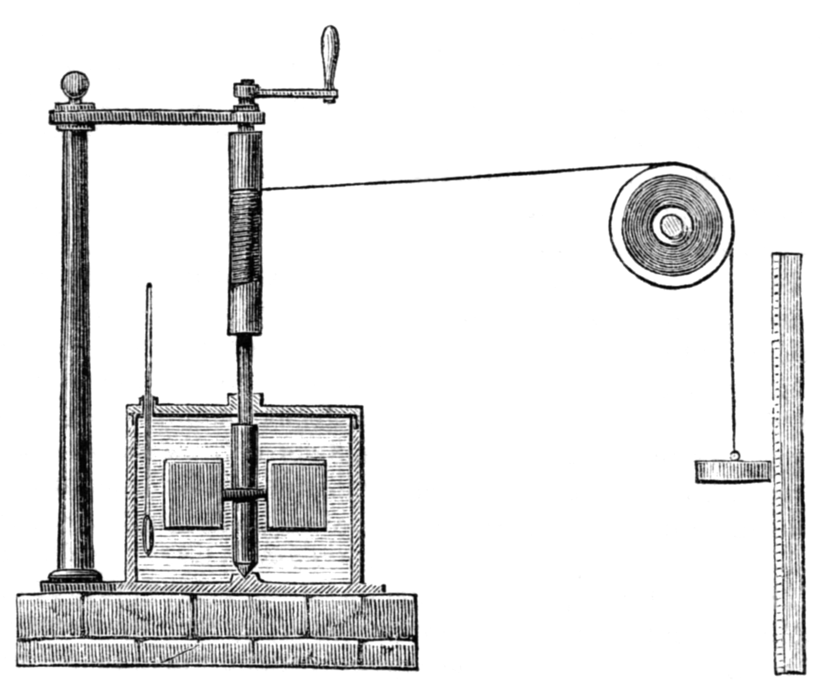
Figure 1:Joule’s apparatus for measuring the mechanical equivalent of heat. The falling weights turn a paddle wheel immersed in water, converting a known amount of mechanical work into a measurable temperature rise. Modern calorimeters (Section 3.3) use the same principle—measuring temperature changes to quantify energy transfers—but with electrical heating in place of falling weights.
In 1847, James Prescott Joule measured how mechanical work converts into heat. He famously found that dropping a total of 778 lbft of weight (e.g., by turning a paddle in water) raised the temperature of 1 lb of water by . Converting to SI units:
Here, is the specific heat of water—i.e., the heat capacity per gram.
First Law of Thermodynamics
Joule’s result showed that a definite quantity of mechanical work always produces the same quantity of heat. This interconvertibility means we need a single energy-conservation statement that accounts for both. To include heat () and work () in one statement of energy conservation, we write
where
is the change in internal energy,
is the heat absorbed by the system,
is the work done on the system.
Differential Form
In differential form,
Rearranging,
This rearranged form is useful because we often want to find the heat exchanged in a process. Since is a state function (calculable from state variables alone) and we can often evaluate from the process path, we can determine by difference.
Types of Work
In Section 1.1, we defined work as “energy transferred when a force acts over a distance.” Mathematically:
Many physical processes fit a “generalized force” “generalized displacement” pattern:
Table 1:Common forms of work as generalized force–displacement pairs
Generalized “Force” | Generalized “Displacement” | Example | |
|---|---|---|---|
Mechanical | Lifting a weight | ||
Linear tension | Stretching a spring | ||
Surface tension | Blowing a soap bubble | ||
Pressure | Compressing a gas | ||
Chemical | or | Forming a molecule | |
Electrical | Charge | Moving an electric charge |
In this course, work () will be our workhorse, but the generalized structure shows up again when we discuss surface phenomena, electrochemistry, and chemical potentials.
Worked Examples
The examples below apply the generalized force–displacement framework from Table 1 to three different work modes: work, surface-tension work, and elastic (spring) work.
Example 1. Expanding Against Constant Pressure
Calculate the work when an ideal gas expands from to against a constant external pressure of .
Solution
Convert Units to SI
Set Up the Work Integral
For a constant external pressure,Perform the Integration
Numerical Result
Interpretation
The negative sign indicates the system (gas) does of work on the surroundings.
According to the convention , if no heat is exchanged (), the gas would lose in internal energy because it expands.
The – diagram below illustrates this process geometrically. The magnitude of the work equals the shaded area under the constant-pressure line.
Source
import numpy as np
import matplotlib.pyplot as plt

fig, ax = plt.subplots(figsize=(5, 3.5))

V_i = 20  # L
V_f = 85  # L
P_ext = 2.5  # bar

# Shaded region: area = |w|
ax.fill_between([V_i, V_f], 0, P_ext, color='C0', alpha=0.25, label=r'$|w| = P_{\mathrm{ext}}\,\Delta V$')

# Constant-pressure line
ax.plot([V_i, V_f], [P_ext, P_ext], 'C0-', lw=2)

# Vertical dashed lines at V_i and V_f
ax.plot([V_i, V_i], [0, P_ext], 'k--', lw=1, alpha=0.5)
ax.plot([V_f, V_f], [0, P_ext], 'k--', lw=1, alpha=0.5)

# Markers for initial and final states
ax.plot(V_i, P_ext, 'ko', ms=6, zorder=5)
ax.plot(V_f, P_ext, 'ko', ms=6, zorder=5)

# Arrow showing direction of expansion
ax.annotate('', xy=(V_f - 2, P_ext + 0.3), xytext=(V_i + 2, P_ext + 0.3),
            arrowprops=dict(arrowstyle='->', color='C3', lw=1.5))
ax.text((V_i + V_f) / 2, P_ext + 0.45, 'expansion', ha='center', fontsize=10, color='C3')

# Labels
ax.text(V_i, -0.25, r'$V_i$', ha='center', fontsize=11)
ax.text(V_f, -0.25, r'$V_f$', ha='center', fontsize=11)
ax.text(2, P_ext, r'$P_{\mathrm{ext}}$', ha='left', va='center', fontsize=11)

ax.set_xlabel('Volume (L)', fontsize=11)
ax.set_ylabel('Pressure (bar)', fontsize=11)
ax.set_xlim(0, 100)
ax.set_ylim(0, 4)
ax.legend(loc='upper right', fontsize=10, framealpha=0.9)
ax.set_title('Constant-Pressure Expansion', fontsize=12)

plt.tight_layout()
plt.show()
plt.close(fig)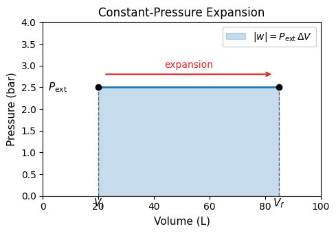
Figure 1 showed how Joule connected mechanical work to heat. Here, the – diagram provides the geometric interpretation of work that we will use throughout this chapter: work equals the area under the pressure curve on a – diagram. Different paths between the same initial and final volumes can enclose different areas, which is precisely why work is path-dependent.
Example 2. Expanding a Soap Bubble
Calculate the work necessary to expand a soap bubble (two surfaces) with surface tension (, the value for a water–air interface at room temperature) from a radius of to .
Source
import numpy as np
import matplotlib.pyplot as plt
from matplotlib.patches import Arc, FancyArrowPatch

fig, ax = plt.subplots(figsize=(5, 4))

# Bubble parameters
center = (0, 0)
r_outer = 2.0
r_inner = 1.8  # thin film
film_thickness = r_outer - r_inner

# Draw the outer surface
theta = np.linspace(0, 2 * np.pi, 300)
ax.plot(r_outer * np.cos(theta), r_outer * np.sin(theta), 'C0-', lw=2.5, label='Outer surface')

# Draw the inner surface
ax.plot(r_inner * np.cos(theta), r_inner * np.sin(theta), 'C1-', lw=2.5, label='Inner surface')

# Shade the film region
theta_fill = np.linspace(0, 2 * np.pi, 300)
ax.fill_between(
    r_outer * np.cos(theta_fill),
    r_outer * np.sin(theta_fill),
    r_inner * np.sin(theta_fill),
    alpha=0.15, color='C0'
)
# Fill the other half of the annulus
ax.fill(
    np.concatenate([r_outer * np.cos(theta_fill), r_inner * np.cos(theta_fill[::-1])]),
    np.concatenate([r_outer * np.sin(theta_fill), r_inner * np.sin(theta_fill[::-1])]),
    alpha=0.2, color='C4', label='Soap film'
)

# Radius arrow to outer surface
angle_deg = 35
angle_rad = np.radians(angle_deg)
ax.annotate(
    '', xy=(r_outer * np.cos(angle_rad), r_outer * np.sin(angle_rad)),
    xytext=center,
    arrowprops=dict(arrowstyle='->', color='k', lw=1.5)
)
# Label r
r_mid = (r_outer * 0.55)
ax.text(r_mid * np.cos(angle_rad) - 0.05, r_mid * np.sin(angle_rad) + 0.12,
        r'$r$', fontsize=14, ha='center', va='bottom')

# Zoom inset showing film thickness
# Draw a magnified bracket on the right side
inset_angle = 0  # radians (right side)
x_outer = r_outer * np.cos(inset_angle)
y_outer = r_outer * np.sin(inset_angle)
x_inner = r_inner * np.cos(inset_angle)
y_inner = r_inner * np.sin(inset_angle)

# Bracket lines for film thickness
bracket_len = 0.4
ax.plot([x_outer, x_outer + bracket_len], [y_outer + 0.05, y_outer + 0.05], 'k-', lw=1)
ax.plot([x_inner, x_inner + bracket_len], [y_inner - 0.05, y_inner - 0.05], 'k-', lw=1)
ax.annotate(
    '', xy=(x_outer + bracket_len - 0.05, y_outer + 0.05),
    xytext=(x_inner + bracket_len - 0.05, y_inner - 0.05),
    arrowprops=dict(arrowstyle='<->', color='k', lw=1.2)
)
ax.text(x_outer + bracket_len + 0.08, (y_outer + y_inner) / 2,
        'film', fontsize=10, ha='left', va='center', style='italic')

# Label "air inside" and "air outside"
ax.text(0, 0, 'air\ninside', fontsize=11, ha='center', va='center', color='0.4')
ax.text(0, -2.55, 'air outside', fontsize=11, ha='center', va='center', color='0.4')

# Surface labels
ax.text(-r_inner - 0.15, 0.8, 'inner\nsurface', fontsize=9, ha='right', va='center', color='C1')
ax.text(-r_outer - 0.15, -0.8, 'outer\nsurface', fontsize=9, ha='right', va='center', color='C0')

# Annotations for areas
ax.text(r_outer + 0.15, 1.4, r'$A_{\mathrm{outer}} = 4\pi r^2$', fontsize=11,
        ha='left', va='center', color='C0',
        bbox=dict(boxstyle='round,pad=0.3', fc='white', ec='C0', alpha=0.8))
ax.text(r_outer + 0.15, -1.4, r'$A_{\mathrm{total}} = 2 \times 4\pi r^2 = 8\pi r^2$', fontsize=11,
        ha='left', va='center', color='C4',
        bbox=dict(boxstyle='round,pad=0.3', fc='white', ec='C4', alpha=0.8))

ax.set_xlim(-3.2, 5.2)
ax.set_ylim(-3.2, 3.2)
ax.set_aspect('equal')
ax.axis('off')
ax.set_title('Cross-section of a soap bubble', fontsize=12)

plt.tight_layout()
plt.show()
plt.close(fig)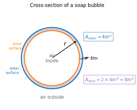
Cross-section of a soap bubble showing the inner and outer surfaces. Because a bubble is a thin film enclosing air, its total surface area is , and the differential area change upon inflation is .
Solution
Convert Units
Identify the Surface Area Change
For a single spherical surface, , so .
A bubble has two surfaces (inner and outer), so its total area is . Hence,
Write the Work Expression
From Table 1, . Here, the surroundings do work on the bubble film to increase its area:Perform the Integral
Substituting for the bubble:Thus,
Calculate Numerically
Evaluating step by step:
Interpretation
The positive sign means the surroundings do work on the system (the bubble film) to increase its surface area. This is consistent with everyday experience: you must blow air (do work) to inflate a soap bubble.
The magnitude is very small (millijoules) because the surface tension of water is modest () and the area change, while geometrically large (), is small in SI units.
Example 3. Stretching a Hookean Fiber
Calculate the work required to stretch a fiber obeying Hooke’s law, with , by .
Solution
Convert Units
Write the Work Expression
Hooke’s law for tension: . The infinitesimal work is:Integrate
If we stretch from to :Substitute Numbers
Interpretation
This is the energy required (work done on the system) to stretch the fiber by .
The positive sign indicates the system absorbs energy (an external force pulls on the fiber).
Note that unlike constant-pressure expansion, the Hookean force varies with displacement, producing the factor of .
Worked Example
Free Expansion of an Ideal Gas
A rigid, insulated container is divided in half by a membrane. One side contains moles of an ideal gas at temperature ; the other side is evacuated. The membrane is punctured. Determine , , and .
Work
The gas expands into vacuum, so :
Heat
The container is insulated (adiabatic walls), so .
Internal energy change
From the First Law:
Result. In free expansion, , , and . For an ideal gas (where depends only on ), this means the temperature does not change either. Free expansion is the extreme case of an irreversible process: the gas does no work and exchanges no heat, yet it undergoes a dramatic change of state (its volume doubles).
Concept Checks
Why are and called path functions while is a state function?
In which sign convention does expansion work appear as positive? How would the First Law be written then?
Why does work depend on the external pressure for irreversible expansions?
What is the physical meaning of the chemical work term ?
Two processes connect the same initial and final states. Process A involves more work than Process B. Which process involves more heat? (Assume only work.)
Key Takeaways
The First Law () enforces energy conservation by bookkeeping heat and work.
Heat and work are path-dependent (, are inexact differentials); internal energy is a state function ( is an exact differential).
Many work modes share a generalized force–displacement structure, including work .
The magnitude of work equals the area under the pressure curve on a – diagram. Different paths between the same states enclose different areas.
Careful sign conventions prevent systematic mistakes in energy balances.