3.2. Applications of the First Law

Overview and Learning Objectives¶

If you heat a gas in a sealed rigid container versus a piston open to the atmosphere, the temperature changes will differ—even for the same amount of heat. Why? The answer lies in how constraints (constant $V$ vs. constant $P$ ) redirect energy between heat and work. This section develops a systematic workflow for applying the First Law under different process constraints, then illustrates it with common ideal-gas cases and a microscopic interpretation.

We begin by clarifying the definitions of quasi-static, reversible, and irreversible processes. We then outline a step-by-step method for using the First Law under different constraints, derive results for isochoric, isothermal, and adiabatic ideal-gas processes, and end with a microscopic interpretation that connects probability distributions of microstates with heat and work.

Learning objectives:

Differentiate quasi-static, reversible, and irreversible processes and explain why reversibility is an idealization.
Explain why reversible expansion produces the maximum work for a given volume change (and reversible compression requires the minimum work).
Rewrite the First Law in terms of chosen independent variables and apply constraints (isothermal, isochoric, isobaric, adiabatic).
Integrate $PV$ work and heat for common ideal-gas processes and relate results to state-variable changes.
Interpret microscopic changes in $p_i$ and $E_i$ as heat and work contributions to $dU$ .

Core Ideas and Derivations¶

Thermodynamic Processes¶

Quasi-static process: A process carried out infinitesimally slowly so that the system remains nearly in equilibrium at all times. Each intermediate state is well-defined thermodynamically.
Reversible process: An idealized process that is (1) quasi-static and (2) free of dissipative effects, meaning it can be reversed with no net change to the system or surroundings.
Irreversible process: Any process that violates one or more of the conditions for reversibility (e.g., too rapid, frictional, or dissipative).
Dissipative effects: Processes that convert ordered energy into disordered (thermal) energy in a way that cannot be undone spontaneously. Common examples include friction, viscous drag, turbulence, electrical resistance, and heat flow across a finite temperature difference.

Examples: Reversible vs. irreversible

Approximately reversible: Slowly compressing a gas in a well-lubricated, frictionless piston, one infinitesimal step at a time. At each step, the system is in mechanical equilibrium with the surroundings ( $P_{\mathrm{int}} \approx P_{\mathrm{ext}}$ ), and the process can be reversed by an infinitesimal decrease in external pressure.

Irreversible: Puncturing a membrane so that a gas undergoes free expansion into vacuum (as in Section 3.1). The gas is never in equilibrium during the expansion—there is no well-defined pressure for the system as a whole—and no infinitesimal change to the surroundings will reverse the process.

Key practical consequence: For a given initial and final state, a reversible expansion does the maximum work on the surroundings ( $|w_{\mathrm{rev}}| \geq |w_{\mathrm{irrev}}|$ for expansion). This is because, at every infinitesimal step, the system pushes against the highest possible opposing pressure ( $P_{\mathrm{ext}} = P$ ), maximizing $\int P\,dV$ .

How to Apply the First Law of Thermodynamics¶

The First Law states (Section 3.1, Eq. (5)):

dU = \delta q + \delta w,

(1)

where $dU$ is the change in internal energy, $\delta q$ is the heat added to the system, and $\delta w$ is the work done on the system. To make this law useful for specific processes, follow the five-step workflow below.

Workflow overview: (1) Choose independent variables → (2) Rewrite the First Law → (3) Apply constraints → (4) Define the system/EOS → (5) Integrate. Click each step for details.

Step 1. Choose Two Independent Variables

For a single-component, single-phase system, specifying two independent variables (plus the amount of substance) completely determines the thermodynamic state.

Convenience: Which variables are easiest to control with your experimental setup?
Necessity: Which variables can you reliably measure or keep constant?
Curiosity: Which variables are most relevant to the phenomenon you wish to explore?

Common choices include $(V, T)$ for gases in rigid containers and $(P, T)$ for processes open to the atmosphere.

Step 2. Rewrite the First Law in Terms of Your Chosen Variables

Start from $\delta q = dU - \delta w$ . For $PV$ -only work, $\delta w = -P\,dV$ , so

\delta q = dU + P\,dV.

(2)

Now expand $dU$ as a total differential in your chosen variables. For example, with $V$ and $T$ :

dU = \left(\frac{\partial U}{\partial T}\right)_V dT + \left(\frac{\partial U}{\partial V}\right)_T dV,

(3)

which gives

\delta q = \left(\frac{\partial U}{\partial T}\right)_V dT + \left[\left(\frac{\partial U}{\partial V}\right)_T + P\right] dV.

(4)

Note that this expression for $\delta q$ has three contributions: the response of $U$ to temperature, the response of $U$ to volume, and the $P\,dV$ work term. This is not just the total differential of $U$ —the work term matters.

Step 3. Apply Constraints

Constant state variables:
- Isobaric ( $dP=0$ ), Isochoric ( $dV=0$ ), Isothermal ( $dT=0$ ).
Adiabatic:
- If the boundary is thermally insulating, $\delta q = 0$ .
- “Adiabatic” means no heat transfer, but the system may still perform or receive work.

Applying a constraint eliminates one or more terms from your Step 2 expression, often making the resulting differential equation separable and integrable.

Step 4. Define the System (Equation of State)

Specify an equation of state if known (e.g., $PV=nRT$ for an ideal gas, or the van der Waals EOS from Section 1.4).
Use the equation of state to evaluate partial derivatives—e.g., $\left(\frac{\partial U}{\partial V}\right)_T = 0$ for an ideal gas—that appear in your expression for $\delta q$ .
This step is where the physics of the system enters: different substances yield different results for the same constraint.

Step 5. Integrate the First Law

Integrate the differential relationships to link total heat ( $q$ ) or work ( $w$ ) to finite changes in state variables.
For reversible processes, the integration path in state space is well-defined.
For irreversible processes, compute $\Delta U$ from state variables (it’s path-independent) and use the First Law to relate $q$ and $w$ .

Applying the Workflow: $V$ and $T$ as Independent Variables¶

For many systems—especially gases—choosing $V$ and $T$ as independent variables simplifies calculations. Let us walk through the five-step workflow for a monatomic ideal gas.

Step 1–2: First Law in Terms of $V$ and $T$ ¶

Starting from

\delta q = dU + P\,dV,

(5)

we rewrite $dU$ as a total differential in $V$ and $T$ :

dU = \left(\frac{\partial U}{\partial T}\right)_V dT \;+\; \left(\frac{\partial U}{\partial V}\right)_T dV.

(6)

Substituting:

\delta q = \underbrace{\left(\frac{\partial U}{\partial T}\right)_V}_{C_V} dT \;+\; \left[\left(\frac{\partial U}{\partial V}\right)_T + P\right] dV.

(7)

Step 4: Ideal-Gas Simplification¶

For an ideal gas, $U$ depends only on $T$ (there are no intermolecular interactions to make $U$ depend on $V$ ), so $\left(\frac{\partial U}{\partial V}\right)_T = 0$ . For a monatomic ideal gas specifically,

U = \frac{3}{2} N k_B T, \quad P = \frac{N k_B T}{V}, \quad C_V = \left(\frac{\partial U}{\partial T}\right)_V = \frac{3}{2} N k_B.

(8)

Equation (7) then simplifies to

\delta q = C_V \, dT + P \, dV \qquad\text{(ideal gas, $PV$-only work).}

(9)

Step 3: Process Constraints¶

Prediction exercise

Before we derive the results, predict which quantities vanish for each process. Fill in the blanks:

Process	$dV = 0$ ?	$dT = 0$ ?	$\delta q = 0$ ?	$\Delta U = ?$
Isochoric heating
Isothermal expansion
Adiabatic expansion

Check your predictions

Process	$dV = 0$ ?	$dT = 0$ ?	$\delta q = 0$ ?	$\Delta U$
Isochoric heating	Yes	No	No	$q$ (= $C_V \Delta T$ )
Isothermal expansion	No	Yes	No	0 (ideal gas)
Adiabatic expansion	No	No	Yes	$w$

Key insight: each constraint eliminates a different term from Equation (9), producing a different relationship among $q$ , $w$ , and state-variable changes.

Applying these constraints to Equation (9):

Table 1:Processes for an Ideal Gas ( $V$ and $T$ as Independents)

Constraint	Condition	Resulting $\delta q$
Isochoric	$dV = 0$	$\delta q = C_V\, dT$
Isothermal	$dT = 0$	$\delta q = P\, dV$
Adiabatic	$\delta q = 0$	$C_V\, dT = -P\, dV$

Step 5: Integrations Under Specific Constraints¶

Isochoric ( $dV = 0$ )
With no volume change, there is no $PV$ work ( $w = 0$ ). All energy enters as heat:
$\delta q = C_V\, dT \quad \Longrightarrow \quad q = \int_{T_1}^{T_2} C_V \, dT = \frac{3}{2} N k_B \,\Delta T.$
(10)
Since $w = 0$ , we also have $\Delta U = q = C_V \Delta T$ .
Isothermal ( $dT = 0$ )
For an ideal gas, $\Delta U = 0$ (because $U$ depends only on $T$ ). The system absorbs heat to offset the work it does:
$q = \int_{V_1}^{V_2} \frac{N k_B T}{V} \, dV = N k_B T \ln\!\bigl(\tfrac{V_2}{V_1}\bigr).$
(11)
And $w = -q = -N k_B T \ln(V_2/V_1)$ .
Adiabatic ( $\delta q = 0$ )
Setting $\delta q = 0$ in Equation (9):
$C_V\, dT = -P\, dV = -\frac{N k_B T}{V}\, dV.$
(12)
Separating variables:
$\frac{C_V}{T}\, dT = -\frac{N k_B}{V}\, dV \quad \Longrightarrow \quad \int_{T_1}^{T_2} \frac{C_V}{T}\, dT = - \int_{V_1}^{V_2} \frac{N k_B}{V}\, dV.$
(13)
Integrating both sides:
$\frac{3}{2} N k_B \ln\frac{T_2}{T_1} = -N k_B \ln\frac{V_2}{V_1}.$
(14)
Dividing through by $N k_B$ :
$\ln\frac{T_2}{T_1} = -\frac{2}{3}\ln\frac{V_2}{V_1} = \ln\!\left(\frac{V_1}{V_2}\right)^{2/3}.$
(15)
Exponentiating:
$\boxed{T_1 V_1^{2/3} = T_2 V_2^{2/3}} \qquad\text{(monatomic ideal gas).}$
(16)
Where does the exponent $2/3$ come from?
The exponent arises from the ratio $N k_B / C_V = N k_B / (\frac{3}{2} N k_B) = 2/3$ . For a general ideal gas, this ratio is $\gamma - 1$ , where $\gamma = C_P / C_V$ is the heat-capacity ratio. The general adiabatic relation is
$T V^{\gamma - 1} = \text{const},$
(17)
which, combined with $PV = nRT$ , also gives $PV^\gamma = \text{const}$ . We will use these relations when we compare isothermal and adiabatic processes below.

Comparing Isothermal and Adiabatic Expansions¶

How does the path affect the work? The $P$ – $V$ diagram below compares a reversible isothermal expansion with a reversible adiabatic expansion from the same initial state. The shaded areas represent $|w|$ for each process.

import numpy as np
import matplotlib.pyplot as plt

# Parameters
n = 1.0        # mol
R = 8.314      # J/(mol K)
T1 = 300       # K
V1 = 5.0e-3    # m^3 (5 L)
V2 = 20.0e-3   # m^3 (20 L)
gamma = 5/3    # monatomic ideal gas

P1 = n * R * T1 / V1  # initial pressure

# Volume array
V = np.linspace(V1, V2, 500)
V_L = V * 1e3  # convert to liters for plotting

# Isothermal: P = nRT/V
P_iso = n * R * T1 / V

# Adiabatic: P V^gamma = P1 V1^gamma  =>  P = P1 (V1/V)^gamma
P_adi = P1 * (V1 / V)**gamma

# Convert pressures to bar for plotting
P_iso_bar = P_iso / 1e5
P_adi_bar = P_adi / 1e5
P1_bar = P1 / 1e5

fig, ax = plt.subplots(figsize=(6, 4))

# Shaded areas
ax.fill_between(V_L, 0, P_iso_bar, alpha=0.15, color='C0', label=r'$|w_{\mathrm{iso}}|$')
ax.fill_between(V_L, 0, P_adi_bar, alpha=0.15, color='C3', label=r'$|w_{\mathrm{adi}}|$')

# Curves
ax.plot(V_L, P_iso_bar, 'C0-', lw=2.5, label=f'Isothermal ($T = {T1}$ K)')
ax.plot(V_L, P_adi_bar, 'C3-', lw=2.5, label=f'Adiabatic ($\\gamma = 5/3$)')

# Initial state marker
ax.plot(V1 * 1e3, P1_bar, 'ko', ms=7, zorder=5)
ax.annotate('  initial state', xy=(V1 * 1e3, P1_bar), fontsize=10, va='center')

# Compute numerical work values for annotation
w_iso = -n * R * T1 * np.log(V2 / V1)  # J
w_adi = (P1 * V1**gamma / (1 - gamma)) * (V2**(1 - gamma) - V1**(1 - gamma))  # J

ax.set_xlabel('Volume (L)', fontsize=11)
ax.set_ylabel('Pressure (bar)', fontsize=11)
ax.set_xlim(4, 22)
ax.set_ylim(0, P1_bar * 1.15)
ax.legend(loc='upper right', fontsize=10, framealpha=0.9)
ax.set_title('Isothermal vs. Adiabatic Expansion from the Same Initial State', fontsize=11)

# Add work annotations
ax.text(14, 1.8, f'$w_{{\\mathrm{{iso}}}} = {w_iso/1e3:.2f}$ kJ', fontsize=10, color='C0',
        bbox=dict(boxstyle='round,pad=0.3', fc='white', ec='C0', alpha=0.8))
ax.text(14, 0.8, f'$w_{{\\mathrm{{adi}}}} = {w_adi/1e3:.2f}$ kJ', fontsize=10, color='C3',
        bbox=dict(boxstyle='round,pad=0.3', fc='white', ec='C3', alpha=0.8))

plt.tight_layout()
plt.show()
plt.close(fig)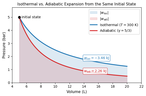

Comparison of reversible isothermal and adiabatic expansions of one mole of a monatomic ideal gas from $(V_1, T_1) = (5\,\mathrm{L}, 300\,\mathrm{K})$ to $V_2 = 20\,\mathrm{L}$ . The isothermal curve lies above the adiabatic curve at every point, so the area under it is larger: isothermal expansion does more work on the surroundings.

Why the difference? During isothermal expansion, heat flows into the gas to maintain a constant temperature, keeping the pressure higher. During adiabatic expansion ( $q = 0$ ), the gas cools as it does work (Eq. (16)), so the pressure drops more steeply. The isothermal path therefore pushes against a higher pressure at every volume increment, producing more work.

Microscopic Interpretation of the First Law¶

As developed in Section 2.1, macroscopic thermodynamic properties are ensemble averages over microstates. This perspective gives a powerful physical picture of heat and work at the molecular level.

From a statistical mechanics perspective, the internal energy is

U = \sum_{i=1}^M p_i E_i,

(18)

where $p_i$ is the probability of occupying the $i$ -th microstate with energy $E_i$ , and $M$ is the total number of accessible microstates. The total differential can be written as

dU = \underbrace{\sum_{i=1}^M E_i\, dp_i}_{\text{changing which states are occupied}} + \underbrace{\sum_{i=1}^M p_i \, dE_i}_{\text{changing the energies of the states}}.

(19)

For a closed system (constant $N$ ) with only $PV$ work, the microstate energies depend on volume. Noting that

\sum_{i=1}^M p_i \left(\frac{\partial E_i}{\partial V}\right)_N = \Bigl\langle \bigl(\tfrac{\partial E}{\partial V}\bigr)_N \Bigr\rangle,

(20)

we identify pressure as

P = - \Bigl\langle \bigl(\tfrac{\partial E}{\partial V}\bigr)_N \Bigr\rangle.

(21)

Hence,

dU = \sum_{i=1}^M E_i\, dp_i \;-\; P\, dV.

(22)

Comparing term by term with $dU = \delta q + \delta w = \delta q - P\,dV$ , we identify:

\delta q = \sum_{i=1}^M E_i\, dp_i \qquad\text{and}\qquad \delta w = -P\,dV = \sum_{i=1}^M p_i\, dE_i.

(23)

The figure below illustrates these two mechanisms. Reading left to right: the initial state, the result of adding heat (probabilities shift; energy levels unchanged), and the result of doing work via compression (energy levels shift; probabilities unchanged).

import numpy as np
import matplotlib.pyplot as plt

N_microstates = 5
E_microstates = np.array([0, 1, 2, 3, 4])
P_microstates = np.array([0.5, 0.3, 0.1, 0.05, 0.05])
P_microstates /= P_microstates.sum()

fig, axs = plt.subplots(1, 3, figsize=(13, 4.5), constrained_layout=True, sharex=True)

# --- Panel 0 (left): Initial state ---
axs[0].set_title('Initial State', fontsize=11, fontweight='bold')

for i in range(N_microstates):
    axs[0].plot([0, 1], [E_microstates[i], E_microstates[i]], color='C0', alpha=0.5, lw=1.5)
    axs[0].fill_betweenx(
        [E_microstates[i], E_microstates[i] + 0.15], 0, P_microstates[i],
        color='C1', alpha=0.5
    )
    axs[0].text(
        P_microstates[i] + 0.02, E_microstates[i] + 0.07,
        f'$p_{i+1}={P_microstates[i]:.2f}$', fontsize=9, ha='left'
    )
axs[0].set_xlabel('Probability')
axs[0].set_ylabel('Energy')
axs[0].set_xlim(0, 0.75)
axs[0].set_ylim(-0.5, 9)

# --- Panel 1 (middle): After heating ---
axs[1].set_title('After Heating ($\\delta q > 0$)\n$\\{p_i\\}$ change; $\\{E_i\\}$ fixed',
                  fontsize=11, fontweight='bold')

P_heated = np.array([0.35, 0.25, 0.18, 0.12, 0.10])
P_heated /= P_heated.sum()

for i in range(N_microstates):
    axs[1].plot([0, 1], [E_microstates[i], E_microstates[i]], color='C0', alpha=0.5, lw=1.5)
    axs[1].fill_betweenx(
        [E_microstates[i], E_microstates[i] + 0.15], 0, P_heated[i],
        color='C3', alpha=0.5
    )
    axs[1].text(
        P_heated[i] + 0.02, E_microstates[i] + 0.07,
        f'$p_{i+1}={P_heated[i]:.2f}$', fontsize=9, ha='left'
    )
axs[1].set_xlabel('Probability')
axs[1].set_xlim(0, 0.75)
axs[1].set_ylim(-0.5, 9)

# --- Panel 2 (right): After compression ---
axs[2].set_title('After Compression ($\\delta w > 0$)\n$\\{E_i\\}$ change; $\\{p_i\\}$ fixed',
                  fontsize=11, fontweight='bold')

E_compressed = np.array([0, 2, 4, 6, 8])

for i in range(N_microstates):
    axs[2].plot([0, 1], [E_compressed[i], E_compressed[i]], color='C0', alpha=0.5, lw=1.5)
    axs[2].fill_betweenx(
        [E_compressed[i], E_compressed[i] + 0.15], 0, P_microstates[i],
        color='C4', alpha=0.5
    )
    axs[2].text(
        P_microstates[i] + 0.02, E_compressed[i] + 0.07,
        f'$p_{i+1}={P_microstates[i]:.2f}$', fontsize=9, ha='left'
    )
axs[2].set_xlabel('Probability')
axs[2].set_xlim(0, 0.75)
axs[2].set_ylim(-0.5, 9)

plt.show()
plt.close(fig)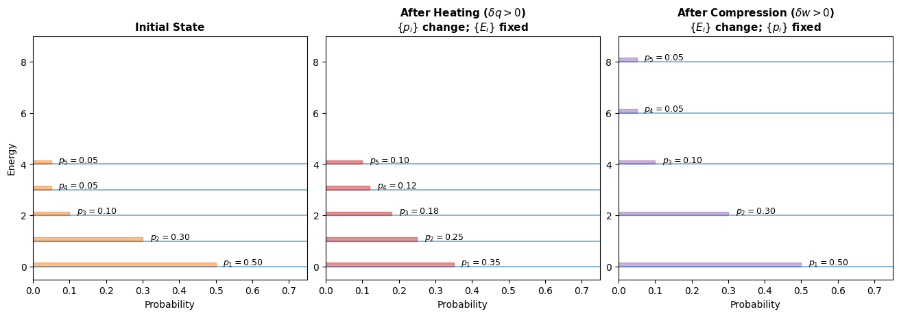

Schematic of microstate energies (vertical axis) and occupation probabilities (horizontal bars). Left: initial state. Middle: after heating—the energy levels are unchanged, but the distribution shifts toward higher-energy states ( $\sum E_i\,dp_i > 0$ ). Right: after compression—the probabilities are unchanged, but every energy level shifts upward ( $\sum p_i\,dE_i > 0$ ).

Think–pair–share

In the microscopic picture, heating at constant volume changes $\{p_i\}$ while $\{E_i\}$ stay fixed (middle panel above). What would the figure look like if you heated at constant pressure instead? Would only the probabilities change, only the energies, or both? Why?

Discussion

Both. At constant pressure, adding heat increases $T$ , which shifts the probability distribution toward higher-energy states (just as at constant $V$ ). But at constant $P$ , the gas also expands, which changes the volume and therefore shifts the energy levels (just as in compression, but in reverse—the levels decrease). At constant pressure, $\delta q$ simultaneously changes both $\{p_i\}$ and $\{E_i\}$ .

This is one reason $C_P > C_V$ : at constant pressure, some of the heat goes into changing energy levels (doing expansion work) rather than solely redistributing probabilities. We will quantify this relationship in Section 3.3.

Worked Example¶

Isothermal reversible expansion of an ideal gas¶

One mole of an ideal gas expands reversibly and isothermally at $T=300\ \mathrm{K}$ from $V_1=5.0\ \mathrm{L}$ to $V_2=20.0\ \mathrm{L}$ . Compute $w$ , $q$ , and $\Delta U$ .

Assumptions. Ideal gas, reversible process, isothermal; for an ideal gas $U=U(T)$ .

Work
For a reversible process, $P_{\mathrm{ext}} = P = nRT/V$ at every step:
$w = -\int_{V_1}^{V_2} P\,dV = -\int_{V_1}^{V_2}\frac{nRT}{V}\,dV = -nRT\ln\left(\frac{V_2}{V_1}\right).$
(24)
With $n=1\,\mathrm{mol}$ , $R=8.314\ \mathrm{J\,mol^{-1}\,K^{-1}}$ , $T=300\ \mathrm{K}$ , and $V_2/V_1=4$ :
$w = -(1)(8.314)(300)\ln 4 = -3.46\times10^{3}\ \mathrm{J}=-3.46\ \mathrm{kJ}.$
(25)
Internal energy
$\Delta U = 0 \quad (\text{isothermal ideal gas: } U = U(T) \text{ and } \Delta T = 0).$
(26)
Heat from the First Law
$\Delta U = q + w \;\Rightarrow\; 0 = q + w \;\Rightarrow\; q = -w = +3.46\ \mathrm{kJ}.$
(27)

Result. $w=-3.46\ \mathrm{kJ}$ , $q=+3.46\ \mathrm{kJ}$ , and $\Delta U=0$ . The gas does work on the surroundings, and an equal amount of heat flows in from the thermal reservoir to maintain the temperature.

Computational check

Verify this result using Python. Compute $w = -nRT\ln(V_2/V_1)$ numerically and confirm it matches the hand calculation. Then plot $P$ vs. $V$ for this isothermal expansion and shade the area under the curve. Does the shaded area match $|w|$ ?

import numpy as np
import matplotlib.pyplot as plt

n = 1.0        # mol
R = 8.314      # J/(mol K)
T = 300        # K
V1 = 5.0e-3    # m^3 (5 L)
V2 = 20.0e-3   # m^3 (20 L)

# Analytical result
w = -n * R * T * np.log(V2 / V1)
print(f"Work (analytical): w = {w:.1f} J = {w/1e3:.3f} kJ")

# Numerical integration (trapezoidal) for verification
V = np.linspace(V1, V2, 10000)
P = n * R * T / V
w_numerical = -np.trapezoid(P, V)
print(f"Work (numerical):  w = {w_numerical:.1f} J = {w_numerical/1e3:.3f} kJ")

# Plot
fig, ax = plt.subplots(figsize=(5, 3.5))
V_L = V * 1e3
P_bar = P / 1e5
ax.fill_between(V_L, 0, P_bar, alpha=0.2, color='C0', label=f'$|w| = {abs(w)/1e3:.2f}$ kJ')
ax.plot(V_L, P_bar, 'C0-', lw=2)
ax.set_xlabel('Volume (L)')
ax.set_ylabel('Pressure (bar)')
ax.set_title('Reversible Isothermal Expansion ($T = 300$ K)')
ax.legend(fontsize=10)
plt.tight_layout()
plt.show()
plt.close(fig)

Work (analytical): w = -3457.7 J = -3.458 kJ
Work (numerical):  w = -3457.7 J = -3.458 kJ

Concept Checks¶

Why is reversibility useful even when real processes are irreversible?
What distinguishes an isothermal process from an adiabatic process in terms of energy transfer mechanisms?
For an ideal gas, why does $\left(\partial U/\partial V\right)_T=0$ ?
In the microscopic expression $dU=\sum_i E_i\,dp_i+\sum_i p_i\,dE_i$ , which term corresponds to heat and which to work (under the stated conditions)?
An isothermal expansion and an adiabatic expansion start from the same initial state and end at the same final volume. Which produces more work? Which produces a larger temperature change?

Key Takeaways¶

Reversible processes serve as idealized benchmarks: reversible expansion maximizes work output; reversible compression minimizes work input.
Choosing independent variables and constraints turns the First Law into solvable differential relations.
Ideal-gas isothermal expansion has $\Delta U=0$ and $q=-w$ .
Adiabatic constraints set $q=0$ and force $T$ to change when work is done; the relation $TV^{\gamma-1} = \text{const}$ governs the temperature–volume coupling.
On a $P$ – $V$ diagram, work equals the area under the curve. Different paths between the same endpoints yield different areas—a visual proof that work is path-dependent.
Microscopically, heat changes the probability distribution over fixed energy levels, while work shifts the energy levels themselves.