3.3. Enthalpy

Overview and Learning Objectives¶

Most chemistry happens at constant pressure—reactions in open beakers, biological processes at atmospheric pressure, industrial reactors vented to the atmosphere. Under these conditions, the heat we measure is not $\Delta U$ but something slightly different: some of the energy goes into $PV$ work as the system expands or contracts against the atmosphere. Enthalpy $H = U + PV$ provides the natural accounting for constant-pressure heat flow, absorbing that $PV$ bookkeeping into a single state function.

This section derives enthalpy from the First Law at constant pressure, relates $q_P$ to $\Delta H$ , introduces the constant-pressure heat capacity $C_P$ , and develops the standard enthalpy framework (formation and reaction enthalpies, Hess’s Law) used throughout thermochemistry.

Learning objectives:

Derive the definition $H=U+PV$ and show that $q_P=\Delta H$ for constant-pressure processes with only $PV$ work.
Distinguish conditions under which $q_P = \Delta H$ holds from those where it does not (e.g., non- $PV$ work at constant pressure).
Define heat capacity at constant pressure $C_P$ and use it to compute enthalpy changes over temperature intervals.
Explain standard states and the meaning of standard enthalpy of formation and reaction.
Apply Hess’s Law to compute $\Delta H_{\mathrm{rxn}}^\circ$ from formation enthalpies.

Core Ideas and Derivations¶

Defining Enthalpy¶

The Problem: $\delta q_V = dU$ Is Nice—Can We Do the Same at Constant $P$ ?¶

In Section 3.2, we saw that at constant volume ( $dV = 0$ ), the First Law simplifies beautifully:

\delta q_V = dU.

(1)

The heat absorbed at constant volume equals the change in a state function ( $U$ ), which means $q_V$ is path-independent for any process between two fixed states at the same volume. This is experimentally powerful: measuring $q$ in a bomb calorimeter (constant $V$ ) directly gives $\Delta U$ .

But most chemistry happens at constant pressure, not constant volume. At constant $P$ , the First Law gives

\delta q_P = dU + P\,dV,

(2)

which involves two terms. Can we define a single state function that plays the same role at constant $P$ that $U$ plays at constant $V$ ? That is, can we find a function $H$ such that $\delta q_P = dH$ ?

Derivation¶

Consider the First Law expression when $T$ and $P$ are the independent variables. Starting from $\delta q = dU + P\,dV$ and writing total differentials of $U(T,P)$ and $V(T,P)$ :

\delta q = \left[\left(\frac{\partial U}{\partial T}\right)_P + P \left(\frac{\partial V}{\partial T}\right)_P\right] dT \;+\; \left[\left(\frac{\partial U}{\partial P}\right)_T + P \left(\frac{\partial V}{\partial P}\right)_T\right] dP.

(3)

At constant pressure ( $dP = 0$ ), this becomes:

\delta q_P = \left[\left(\frac{\partial U}{\partial T}\right)_P + P \left(\frac{\partial V}{\partial T}\right)_P\right] dT.

(4)

The coefficient of $dT$ is what we call the heat capacity at constant pressure:

C_P \;=\; \left(\frac{\partial U}{\partial T}\right)_P \;+\; P \left(\frac{\partial V}{\partial T}\right)_P.

(5)

We seek a state function $H$ such that

\delta q_P = \left(\frac{\partial H}{\partial T}\right)_P \, dT = dH \quad\text{(at constant }P\text{)}.

(6)

Comparing Equations (4) and (6), we need $(\partial H/\partial T)_P = C_P$ . This motivates the definition of enthalpy:

\boxed{H \;=\; U + PV.}

(7)

Verification:

H = U + PV

yields

\delta q_P = dH

Taking the total differential of $H = U + PV$ at constant $P$ :

\begin{align*} \left(\frac{\partial H}{\partial T}\right)_P &= \frac{\partial}{\partial T} \bigl(U + PV\bigr)\bigg|_P \\[6pt] &= \left(\frac{\partial U}{\partial T}\right)_P + P \left(\frac{\partial V}{\partial T}\right)_P + V \underbrace{\left(\frac{\partial P}{\partial T}\right)_P}_{=\,0} \\[6pt] &= \left(\frac{\partial U}{\partial T}\right)_P \;+\; P \left(\frac{\partial V}{\partial T}\right)_P \;=\; C_P. \end{align*}

(8)

This matches Equation (5), confirming that $\delta q_P = C_P\,dT = (\partial H/\partial T)_P\,dT = dH$ at constant pressure. ✓

Measuring Enthalpy and Enthalpy Changes¶

At constant pressure (with $PV$ -only work), the heat absorbed or released by a process equals the change in enthalpy:

q_P = \Delta H = H(T_f) - H(T_i).

(10)

If $C_P$ is approximately constant over the temperature range $\Delta T = T_f - T_i$ , then

\Delta H = \int_{T_i}^{T_f} C_P(T)\,dT \;\approx\; C_P \,\Delta T.

(11)

Calorimetry¶

A typical way to measure $\Delta H$ experimentally is via calorimetry—measuring the temperature change of a known mass of material (often water) that exchanges heat with the process of interest.

import numpy as np
import matplotlib.pyplot as plt
from matplotlib.patches import Rectangle

fig, ax = plt.subplots(figsize=(5.5, 5))

# --- Outer container (insulating walls) ---
outer = Rectangle((0.3, 0.2), 3.4, 3.2, linewidth=2.5, edgecolor='0.4',
                   facecolor='0.92', linestyle='--', label='Insulating walls')
ax.add_patch(outer)

# --- Inner container ---
inner = Rectangle((0.6, 0.4), 2.8, 2.6, linewidth=2, edgecolor='k', facecolor='white')
ax.add_patch(inner)

# --- Water ---
water = Rectangle((0.6, 0.4), 2.8, 2.1, linewidth=0, facecolor='#a8d8ea', alpha=0.6)
ax.add_patch(water)
ax.text(1.1, 1.2, 'Water\n(known mass,\nknown $C_P$)', fontsize=10, ha='center',
        va='center', color='#1a5276', style='italic')

# --- Sample container ---
sample = Rectangle((2.2, 0.5), 0.9, 0.7, linewidth=1.8, edgecolor='C1', facecolor='#fdebd0')
ax.add_patch(sample)
ax.text(2.65, 0.85, 'Sample', fontsize=9, ha='center', va='center',
        fontweight='bold', color='C1')

# --- Thermometer ---
ax.plot([0.85, 0.85], [2.1, 3.3], color='red', lw=3, solid_capstyle='round')
ax.plot([0.85], [2.1], 'ro', ms=8, zorder=5)
ax.text(0.85, 3.45, 'Thermometer', fontsize=9, ha='center', va='bottom', color='red')

# --- Stirrer ---
ax.plot([1.6, 1.6], [1.6, 3.3], 'k-', lw=2)
ax.plot([1.4, 1.6, 1.8], [1.55, 1.4, 1.55], 'k-', lw=2)
ax.text(1.6, 3.45, 'Stirrer', fontsize=9, ha='center', va='bottom', color='0.3')

# --- Heat flow arrow ---
ax.annotate('', xy=(2.15, 1.5), xytext=(2.65, 1.25),
            arrowprops=dict(arrowstyle='->', color='C3', lw=2.5,
                           connectionstyle='arc3,rad=-0.2'))
ax.text(2.75, 1.55, '$q_P$', fontsize=13, color='C3', fontweight='bold')

# --- Labels ---
ax.text(2.0, -0.05, 'Constant-pressure calorimeter (schematic)', fontsize=11,
        ha='center', va='top', fontweight='bold')
ax.text(3.85, 1.8, 'insulating\nwalls', fontsize=8, ha='center', va='center',
        color='0.4', style='italic', rotation=90)

ax.set_xlim(-0.1, 4.3)
ax.set_ylim(-0.2, 3.7)
ax.set_aspect('equal')
ax.axis('off')

plt.tight_layout()
plt.show()
plt.close(fig)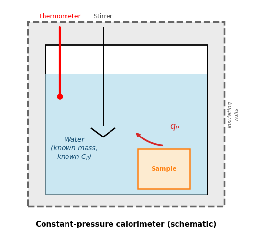

Schematic of a constant-pressure calorimeter. The reaction occurs in the sample container; the released or absorbed heat ( $q_P$ ) flows into the surrounding water, producing a measurable temperature change. Insulating walls minimize heat loss to the room. Since the process occurs at atmospheric pressure, $q_P = \Delta H$ .

In-class activity

Dissolving ammonium nitrate ( $\text{NH}_4\text{NO}_3$ ) in water is endothermic—this is the chemistry behind instant cold packs. Suppose you dissolve $10\,\mathrm{g}$ of $\text{NH}_4\text{NO}_3$ ( $M = 80.04\,\mathrm{g/mol}$ ) in $100\,\mathrm{mL}$ of water in a Styrofoam cup and measure a temperature drop of $5.3\,\text{°C}$ .

Estimate $\Delta H_{\mathrm{soln}}$ per mole of $\text{NH}_4\text{NO}_3$ . Assume $C_{P,\mathrm{soln}} \approx C_{P,\mathrm{water}} = 4.18\,\mathrm{J\,g^{-1}\,K^{-1}}$ and that the total solution mass is $\approx 110\,\mathrm{g}$ .

Solution

Heat absorbed by the dissolution process:
The solution cools, so heat flows from the water into the dissolving salt. From the water’s perspective:
$q_{\mathrm{soln}} = -q_{\mathrm{water}} = -m_{\mathrm{soln}}\,C_P\,\Delta T = -(110)(4.18)(-5.3) = +2{,}437\,\mathrm{J}.$
(12)
The positive sign confirms an endothermic process (the system absorbs heat from the water).
Moles of $\text{NH}_4\text{NO}_3$ :
$n = \frac{10\,\mathrm{g}}{80.04\,\mathrm{g/mol}} = 0.125\,\mathrm{mol}.$
(13)
Molar enthalpy of solution:
$\Delta H_{\mathrm{soln}} = \frac{q_P}{n} = \frac{2{,}437}{0.125}\,\mathrm{J/mol} \approx +19.5\,\mathrm{kJ/mol}.$
(14)

The literature value is about $+25.7\,\mathrm{kJ/mol}$ ; the discrepancy comes from heat loss to the surroundings (Styrofoam is not a perfect insulator) and the approximation that $C_{P,\mathrm{soln}} = C_{P,\mathrm{water}}$ .

Defining Common Enthalpy Changes¶

Standard Conditions¶

Standard conditions are defined as $P^\circ = 1\text{ bar}$ . The superscript ° denotes a standard-state quantity (see Notation). Reference databases—e.g., the NIST-JANAF Thermochemical Tables and Active Thermochemical Tables—typically tabulate properties at $T = 25\,\text{°C}$ (298.15 K), though standard-state quantities can be defined at any temperature.

Standard Enthalpy of Formation¶

The standard enthalpy of formation, $\Delta H_f^\circ$ , is the enthalpy change when 1 mole of a compound is formed from its constituent elements in their standard states.

The standard state of an element is its most stable form at $P^\circ = 1\text{ bar}$ (and a specified $T$ ).
By convention, $\Delta H_f^\circ$ for an element in its standard state is zero. This establishes a common reference point for all enthalpy comparisons.

Table 1:Standard States of the Elements

Standard State	Elements
Monatomic ideal gas	He, Ne, Ar, Kr, Xe, Rn
Homonuclear diatomic ideal gas	H, N, O, F, Cl
Liquid	Br, Hg
Solid (most stable crystal structure)	All other elements

The key principle is that the standard state is the most thermodynamically stable form at $P^\circ$ . For most elements this is a solid (e.g., C as graphite, not diamond; Fe as bcc iron). The noble gases are monatomic, the common nonmetals form diatomics, and Br and Hg are liquids at 298 K.

Detailed solid standard states by crystal structure

For reference, the specific crystal structures defining the standard state of each solid element:

Crystal Structure	Elements
Body-centered cubic	Alkali metals (Li, Na, K, Rb, Cs), Ba, group 5 transition metals (V, Nb, Ta), group 6 transition metals (Cr, Mo, W), Mn, Fe, & Eu
Hexagonal	Be, Mg, group 3 transition metals (Sc, Y, Lu), group 4 transition metals (Ti, Zr, Hf), Tc, Re, Ru, Os, Co, group 12 transition metals (Zn, Cd), Tl, C (graphite), Se, Te, most lanthanides (La, Ce, Pr, Nd, Pm, Gd, Tb, Dy, Ho, Er, Tm)
Face-centered cubic	Ca, Sr, Rh, Ir, group 10 transition metals (Ni, Pd, Pt), group 11 transition metals (Cu, Ag, Au), Al, Si (diamond cubic), Ge (diamond cubic), Pb, Yb
Rhombohedral	B, As, Sb, Bi, Sm
Orthorhombic	Ga, P (black), S, I, U, and others
Body-centered tetragonal	In, Sn ( $\beta$ , white)
Simple cubic	Po

Standard Enthalpy of Reaction¶

The standard enthalpy of reaction, $\Delta H_{\mathrm{rxn}}^\circ$ , is the enthalpy change when a reaction is carried out under standard conditions. Mathematically:

\Delta H_{\mathrm{rxn}}^\circ \;=\;\sum_{\text{products}} \nu_p \,H_p^\circ \;-\; \sum_{\text{reactants}} \nu_r \,H_r^\circ,

(15)

where $\nu_p$ and $\nu_r$ are the (positive) stoichiometric coefficients of products and reactants, respectively.

Hess’s Law & Standard Enthalpies of Formation

Hess’s Law: Because enthalpy is a state function, enthalpy changes are additive and path independent. The enthalpy change for a reaction depends only on the initial and final states, not on the route taken between them.

As a consequence, $\Delta H_{\mathrm{rxn}}^\circ$ can be computed from tabulated formation enthalpies:

\Delta H_{\mathrm{rxn}}^\circ \;=\; \sum_{p} \nu_p \,\Delta H_{f,p}^\circ \;-\;\sum_{r} \nu_r \,\Delta H_{f,r}^\circ.

(16)

Alternative notation with signed stoichiometric coefficients

Some texts use signed stoichiometric coefficients $\nu_i$ , defined as positive for products and negative for reactants. In that convention, Hess’s Law takes the compact form

\Delta H_{\mathrm{rxn}}^\circ = \sum_{i} \nu_i \,\Delta H_{f,i}^\circ.

(17)

Both forms are equivalent. For example, in the reaction $\text{CH}_4(g) + 2\,\text{O}_2(g) \to \text{CO}_2(g) + 2\,\text{H}_2\text{O}(g)$ , the signed coefficients are $\nu_{\text{CH}_4} = -1$ , $\nu_{\text{O}_2} = -2$ , $\nu_{\text{CO}_2} = +1$ , $\nu_{\text{H}_2\text{O}} = +2$ .

Example: Steam–Methane Reforming¶

Consider the steam–methane reforming reaction:

\text{CH}_4(g) + \text{H}_2\text{O}(g) \;\;\longrightarrow\;\; \text{CO}(g) + 3\,\text{H}_2(g).

(18)

Applying Equation (16):

\Delta H_{\mathrm{rxn}}^\circ = \Bigl[\Delta H_{f}^\circ(\text{CO}) + 3\,\underbrace{\Delta H_{f}^\circ(\text{H}_2)}_{=\,0}\Bigr] - \Bigl[\Delta H_{f}^\circ(\text{CH}_4) + \Delta H_{f}^\circ(\text{H}_2\text{O})\Bigr].

(19)

Note that $\Delta H_f^\circ(\text{H}_2) = 0$ because $\text{H}_2(g)$ is hydrogen’s standard state.

Alternatively, we can see why this works by decomposing the reaction into formation steps:

Either approach gives the same result, thanks to Hess’s Law.

The enthalpy-level diagram below visualizes the path independence that underlies Hess’s Law. The direct route (left arrow) and the stepwise route through the elements (right arrows) connect the same initial and final states, so they produce the same $\Delta H_{\mathrm{rxn}}^\circ$ .

import numpy as np
import matplotlib.pyplot as plt

fig, ax = plt.subplots(figsize=(7, 5))

# Enthalpy levels (schematic, not to scale)
# Elements at zero reference
y_elements = 0.0
y_reactants = -1.5   # CH4 + H2O are below elements (negative DeltaHf)
y_products = -0.4     # CO + 3H2 are below elements but above reactants

x_left = 1.0
x_right = 5.0
x_mid = 3.0
bar_half = 0.8

# Horizontal bars
bar_kw = dict(lw=2.5, solid_capstyle='butt')
ax.plot([x_left - bar_half, x_left + bar_half], [y_reactants, y_reactants], 'C0-', **bar_kw)
ax.plot([x_right - bar_half, x_right + bar_half], [y_products, y_products], 'C3-', **bar_kw)
ax.plot([x_mid - 1.2, x_mid + 1.2], [y_elements, y_elements], '0.5', **bar_kw, linestyle='--')

# Labels on bars
ax.text(x_left, y_reactants - 0.18, r'$\mathrm{CH_4(g) + H_2O(g)}$',
        fontsize=10, ha='center', va='top', color='C0', fontweight='bold')
ax.text(x_left, y_reactants + 0.12, 'Reactants', fontsize=9, ha='center', va='bottom',
        color='C0')

ax.text(x_right, y_products - 0.18, r'$\mathrm{CO(g) + 3\,H_2(g)}$',
        fontsize=10, ha='center', va='top', color='C3', fontweight='bold')
ax.text(x_right, y_products + 0.12, 'Products', fontsize=9, ha='center', va='bottom',
        color='C3')

ax.text(x_mid, y_elements + 0.12,
        r'Elements in standard states: C(s,graphite), H$_2$(g), O$_2$(g)',
        fontsize=9, ha='center', va='bottom', color='0.4')

# --- Direct arrow (left side) ---
ax.annotate('',
            xy=(x_left + 0.15, y_products + 0.55),
            xytext=(x_left + 0.15, y_reactants + 0.05),
            arrowprops=dict(arrowstyle='->', color='C2', lw=2.5))
ax.text(x_left - 0.65, (y_reactants + y_products) / 2,
        r'$\Delta H_{\mathrm{rxn}}^\circ$' + '\n(direct)',
        fontsize=11, ha='center', va='center', color='C2', fontweight='bold')

# --- Stepwise arrows (right side, through elements) ---
# Reactants -> Elements (go up: reverse formation)
ax.annotate('',
            xy=(x_mid - 0.4, y_elements - 0.05),
            xytext=(x_left + bar_half + 0.1, y_reactants + 0.05),
            arrowprops=dict(arrowstyle='->', color='C1', lw=2,
                           connectionstyle='arc3,rad=-0.15'))
ax.text(1.85, (y_reactants + y_elements) / 2 + 0.25,
        r'$-\sum \nu_r \Delta H_{f,r}^\circ$',
        fontsize=10, ha='center', va='center', color='C1',
        bbox=dict(boxstyle='round,pad=0.2', fc='white', ec='C1', alpha=0.8))

# Elements -> Products (go down: formation)
ax.annotate('',
            xy=(x_right - bar_half - 0.1, y_products + 0.05),
            xytext=(x_mid + 0.4, y_elements - 0.05),
            arrowprops=dict(arrowstyle='->', color='C4', lw=2,
                           connectionstyle='arc3,rad=-0.15'))
ax.text(4.15, (y_elements + y_products) / 2 + 0.15,
        r'$+\sum \nu_p \Delta H_{f,p}^\circ$',
        fontsize=10, ha='center', va='center', color='C4',
        bbox=dict(boxstyle='round,pad=0.2', fc='white', ec='C4', alpha=0.8))

# y-axis label
ax.annotate('', xy=(-0.2, 1.0), xytext=(-0.2, -1.8),
            arrowprops=dict(arrowstyle='->', color='k', lw=1.5))
ax.text(-0.35, -0.4, '$H$', fontsize=14, ha='center', va='center', rotation=90)

ax.set_xlim(-0.8, 6.5)
ax.set_ylim(-2.1, 1.3)
ax.set_aspect('equal')
ax.axis('off')

plt.tight_layout()
plt.show()
plt.close(fig)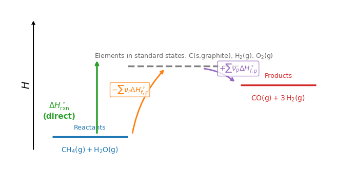

Enthalpy-level diagram for the steam–methane reforming reaction. The direct path (green arrow, left) and the stepwise path through the elements (orange and teal arrows, right) both connect reactants to products. Because $H$ is a state function, both paths give the same $\Delta H_{\mathrm{rxn}}^\circ$ . This is Hess’s Law.

Synthesis: The First Law Toolkit So Far¶

Enthalpy completes our First Law toolkit for the most common laboratory conditions:

Constraint	Relevant state function	Key relation
Constant $V$ (bomb calorimeter)	$U$	$q_V = \Delta U$
Constant $P$ (open beaker, coffee-cup calorimeter)	$H = U + PV$	$q_P = \Delta H$

Hess’s Law lets us combine tabulated formation data to predict $\Delta H_{\mathrm{rxn}}^\circ$ for any reaction without measuring it directly. In the next section, we will see how the temperature dependence of $\Delta H$ (via $C_P$ ) allows us to extrapolate thermochemical data to non-standard temperatures—an essential tool for real-world applications where reactions rarely occur at exactly 298 K.

Try it: Hess’s Law practice

Compute $\Delta H_{\mathrm{rxn}}^\circ$ for the combustion of methane:

\text{CH}_4(g) + 2\,\text{O}_2(g) \longrightarrow \text{CO}_2(g) + 2\,\text{H}_2\text{O}(g).

(22)

Use the following standard enthalpies of formation:

Species	$\Delta H_f^\circ$ (kJ/mol)
CH₄(g)	-74.8
CO₂(g)	-393.5
H₂O(g)	-241.8
O₂(g)	0 (element in standard state)

Set up the Hess’s Law calculation before checking the solution.

Solution

Applying Equation (16):

\Delta H_{\mathrm{rxn}}^\circ = \bigl[\Delta H_f^\circ(\text{CO}_2) + 2\,\Delta H_f^\circ(\text{H}_2\text{O})\bigr] - \bigl[\Delta H_f^\circ(\text{CH}_4) + 2\,\underbrace{\Delta H_f^\circ(\text{O}_2)}_{=\,0}\bigr].

(23)

Substituting numerical values:

\Delta H_{\mathrm{rxn}}^\circ = \bigl[(-393.5) + 2(-241.8)\bigr] - \bigl[(-74.8) + 0\bigr]

(24)

= (-393.5 - 483.6) - (-74.8)

(25)

= -877.1 + 74.8 = \boxed{-802.3\,\mathrm{kJ/mol}}.

(26)

The large negative value confirms that methane combustion is strongly exothermic, consistent with its use as a fuel. Note that $\Delta H_f^\circ(\text{O}_2) = 0$ because O₂(g) is oxygen’s standard state.

Worked Example¶

Heating at constant pressure¶

A sample of liquid water ( $n = 1\,\mathrm{mol}$ ) has constant-pressure heat capacity $C_P=75.0\ \mathrm{J\,mol^{-1}\,K^{-1}}$ (approximately constant over the range). Find $\Delta H$ when it is heated from $T_i=298\ \mathrm{K}$ to $T_f=350\ \mathrm{K}$ at constant pressure.

Setup. At constant pressure with $PV$ -only work, $q_P = \Delta H$ (Eq. (10)), and the enthalpy change is given by Eq. (11):

\Delta H = \int_{T_i}^{T_f} C_P\,dT \approx C_P\,(T_f - T_i).

(27)

Calculation.

\Delta T = 350 - 298 = 52\ \mathrm{K},

(28)

\Delta H \approx (75.0\,\mathrm{J\,mol^{-1}\,K^{-1}})(52\,\mathrm{K}) = 3.90\times10^{3}\ \mathrm{J\,mol^{-1}} = 3.90\ \mathrm{kJ\,mol^{-1}}.

(29)

Result. $\Delta H \approx 3.9\ \mathrm{kJ\,mol^{-1}}$ for this heating step at constant pressure. Because this is a constant-pressure process, this is also the heat absorbed: $q_P = 3.9\,\mathrm{kJ/mol}$ .

Concept Checks¶

Why does adding the $PV$ term make $H$ especially convenient at constant pressure?
When is it not valid to identify $q_P$ with $\Delta H$ ? Give a specific physical example.
Why are formation enthalpies of elements in their standard states defined as zero?
How does Hess’s Law justify computing reaction enthalpies without specifying a mechanism?
Is $C_P$ larger or smaller than $C_V$ for an ideal gas? Why? (Hint: think about what happens to the volume at constant $P$ when you add heat.)

Key Takeaways¶

Enthalpy is defined by $H=U+PV$ and satisfies $q_P=\Delta H$ for constant-pressure processes with $PV$ -only work.
Defining $H$ is an example of a general thermodynamic strategy: when the natural variables for a problem don’t match your existing state function, define a new one. We will use this strategy again for the Helmholtz and Gibbs free energies.
Heat capacities relate temperature changes to enthalpy changes via $\Delta H=\int C_P\,dT$ .
Standard enthalpy changes (formation, reaction) provide a consistent bookkeeping framework. The key convention is $\Delta H_f^\circ = 0$ for elements in their standard states.
Hess’s Law—a direct consequence of $H$ being a state function—lets you build $\Delta H_{\mathrm{rxn}}^\circ$ from tabulated formation enthalpies without knowing the reaction mechanism.

References¶

Thomas C. Allison. (2013). NIST-JANAF Thermochemical Tables - SRD 13. National Institute of Standards. 10.18434/T42S31