7.1. Equilibrium Constant
Course-wide Conventions & Notation
Overview and Learning Objectives ¶ Chapter 6 treated one kind of equilibrium — the coexistence of two phases of a single substance — and showed that the condition for equilibrium reduces to equality of chemical potentials, μ α = μ β \mu_\alpha = \mu_\beta μ α = μ β Chemical equilibrium is the multi-species generalization: instead of two phases of one substance, we now have several chemical species interconverting through a reaction, and the analogous condition (derived below) is
∑ i ν i μ i = 0. \sum_i \nu_i\,\mu_i = 0. i ∑ ν i μ i = 0. In this section we translate that abstract condition into the quantitative tools students have seen in general chemistry: the extent of reaction ξ \xi ξ Q p Q_p Q p K K K
A reaction at constant T , P T,P T , P decreases the Gibbs free energy of the system.
We track progress with the extent of reaction ξ \xi ξ
At constant T T T P P P
( ∂ G ∂ ξ ) T , P = 0. \left(\frac{\partial G}{\partial \xi}\right)_{T,P}=0. ( ∂ ξ ∂ G ) T , P = 0. This minimization gives the chemical equilibrium condition Δ r G = 0 \Delta_r G=0 Δ r G = 0
Δ r G = Δ r G ∘ + R T ln Q p , Δ r G ∘ = − R T ln K . \Delta_r G = \Delta_r G^{\circ} + RT\ln Q_p,
\qquad
\Delta_r G^{\circ} = -RT\ln K. Δ r G = Δ r G ∘ + RT ln Q p , Δ r G ∘ = − RT ln K . The symbol Q Q Q Q p Q_p Q p reaction quotient to distinguish it from the canonical partition function Q ( T , V , N ) Q(T,V,N) Q ( T , V , N ) course-wide notation page for the global convention.
Learning objectives:
Use the extent of reaction ξ \xi ξ d n i = ν i d ξ dn_i=\nu_i\,d\xi d n i = ν i d ξ
Derive Δ r G = ∑ i ν i μ i \Delta_r G=\sum_i \nu_i\mu_i Δ r G = ∑ i ν i μ i ( ∂ G / ∂ ξ ) T , P = Δ r G (\partial G/\partial\xi)_{T,P}=\Delta_r G ( ∂ G / ∂ ξ ) T , P = Δ r G
Derive Δ r G = Δ r G ∘ + R T ln Q p \Delta_r G=\Delta_r G^\circ + RT\ln Q_p Δ r G = Δ r G ∘ + RT ln Q p Q p Q_p Q p
Use Δ r G ∘ = − R T ln K \Delta_r G^\circ=-RT\ln K Δ r G ∘ = − RT ln K Q p Q_p Q p K K K
Apply the van’t Hoff equation to predict how K K K
Core Ideas and Derivations ¶ 7.1.1 Extent of reaction ξ \xi ξ ¶ Consider a general reaction written with stoichiometric coefficients:
ν A A + ν B B ⇌ ν Y Y + ν Z Z . \nu_A A + \nu_B B \rightleftharpoons \nu_Y Y + \nu_Z Z. ν A A + ν B B ⇌ ν Y Y + ν Z Z . A convenient way to describe composition changes is the extent of reaction ξ \xi ξ n i , 0 n_{i,0} n i , 0
n A = n A , 0 − ν A ξ , n B = n B , 0 − ν B ξ , n Y = n Y , 0 + ν Y ξ , n Z = n Z , 0 + ν Z ξ . n_A = n_{A,0} - \nu_A\,\xi,\qquad
n_B = n_{B,0} - \nu_B\,\xi,\qquad
n_Y = n_{Y,0} + \nu_Y\,\xi,\qquad
n_Z = n_{Z,0} + \nu_Z\,\xi. n A = n A , 0 − ν A ξ , n B = n B , 0 − ν B ξ , n Y = n Y , 0 + ν Y ξ , n Z = n Z , 0 + ν Z ξ . Differentiating gives the compact relation
d n i = ν i d ξ dn_i = \nu_i\,d\xi d n i = ν i d ξ if we adopt the signed stoichiometry convention : ν i < 0 \nu_i<0 ν i < 0 ν i > 0 \nu_i>0 ν i > 0
Equation (6) ν i \nu_i ν i Δ r G ≡ ∑ i ν i μ i \Delta_r G \equiv \sum_i \nu_i \mu_i Δ r G ≡ ∑ i ν i μ i Δ ν ≡ ∑ i ν i \Delta \nu \equiv \sum_i \nu_i Δ ν ≡ ∑ i ν i
7.1.2 Gibbs free energy and the equilibrium condition ¶ Treat the system Gibbs energy as a function of T , P T,P T , P
G = G ( T , P , n A , n B , n Y , n Z , … ) . G = G(T,P,n_A,n_B,n_Y,n_Z,\ldots). G = G ( T , P , n A , n B , n Y , n Z , … ) . Its total differential is
d G = ( ∂ G ∂ T ) P , n d T + ( ∂ G ∂ P ) T , n d P + ∑ i ( ∂ G ∂ n i ) T , P , n j ≠ i d n i . dG = \left(\frac{\partial G}{\partial T}\right)_{P,n}\! dT
+ \left(\frac{\partial G}{\partial P}\right)_{T,n}\! dP
+ \sum_i \left(\frac{\partial G}{\partial n_i}\right)_{T,P,n_{j\neq i}} dn_i. d G = ( ∂ T ∂ G ) P , n d T + ( ∂ P ∂ G ) T , n d P + i ∑ ( ∂ n i ∂ G ) T , P , n j = i d n i . The partial derivative ( ∂ G / ∂ n i ) T , P , n j ≠ i \left(\partial G/\partial n_i\right)_{T,P,n_{j\ne i}} ( ∂ G / ∂ n i ) T , P , n j = i chemical potential μ i \mu_i μ i
d G = − S d T + V d P + ∑ i μ i d n i . dG = -S\,dT + V\,dP + \sum_i \mu_i\,dn_i. d G = − S d T + V d P + i ∑ μ i d n i . At constant T T T P P P
d G = ∑ i μ i d n i . dG = \sum_i \mu_i\,dn_i. d G = i ∑ μ i d n i . Using Eq. (6)
d G = ( ∑ i ν i μ i ) d ξ . dG = \left(\sum_i \nu_i\mu_i\right)d\xi. d G = ( i ∑ ν i μ i ) d ξ . This motivates the definition of the Gibbs free energy of reaction :
Δ r G ≡ ∑ i ν i μ i \boxed{\Delta_r G \equiv \sum_i \nu_i\,\mu_i} Δ r G ≡ i ∑ ν i μ i and therefore
( ∂ G ∂ ξ ) T , P = Δ r G . \left(\frac{\partial G}{\partial \xi}\right)_{T,P} = \Delta_r G. ( ∂ ξ ∂ G ) T , P = Δ r G . Spontaneity and equilibrium (constant T , P T,P T , P ¶ Δ r G < 0 \Delta_r G < 0 Δ r G < 0 forward (toward products).
Δ r G = 0 \Delta_r G = 0 Δ r G = 0 equilibrium .
Δ r G > 0 \Delta_r G > 0 Δ r G > 0 backward (toward reactants).
At equilibrium,
Δ r G = 0. \boxed{\Delta_r G = 0.} Δ r G = 0. This is the multi-species analog of the phase-equilibrium condition μ α = μ β \mu_\alpha = \mu_\beta μ α = μ β G G G T , P T,P T , P
7.1.3 Reaction quotient Q p Q_p Q p K K K ¶ To connect Δ r G \Delta_r G Δ r G
Ideal-gas chemical potential ¶ Section 5.3 showed that for one mole of an ideal gas at constant T T T d G = V d P dG = V\,dP d G = V d P P ∘ P^\circ P ∘ P P P G ( T , P ) − G ∘ ( T ) = R T ln ( P / P ∘ ) G(T,P) - G^\circ(T) = RT\ln(P/P^\circ) G ( T , P ) − G ∘ ( T ) = RT ln ( P / P ∘ ) mixture , the same argument with P i P_i P i P P P
μ i ( T , P i ) = μ i ∘ ( T ) + R T ln ( P i P ∘ ) , \mu_i(T,P_i)=\mu_i^{\circ}(T)+RT\ln\left(\frac{P_i}{P^{\circ}}\right), μ i ( T , P i ) = μ i ∘ ( T ) + RT ln ( P ∘ P i ) , where P ∘ P^{\circ} P ∘ notation conventions ) and μ i ∘ ( T ) \mu_i^{\circ}(T) μ i ∘ ( T )
Any logarithm in thermodynamics must take a dimensionless argument. That’s why we never write ln P \ln P ln P ln ( P / P ∘ ) \ln(P/P^\circ) ln ( P / P ∘ ) P ∘ P^\circ P ∘ standard-state pressure (1 bar here).
Numerical example. Take a gas with partial pressure P i = 2.50 bar P_i = 2.50\ \text{bar} P i = 2.50 bar T = 298 K T=298\ \text{K} T = 298 K P ∘ = 1.00 bar P^\circ = 1.00\ \text{bar} P ∘ = 1.00 bar
P i P ∘ = 2.50 bar 1.00 bar = 2.50 (dimensionless) . \frac{P_i}{P^\circ}=\frac{2.50\ \text{bar}}{1.00\ \text{bar}}=2.50 \quad \text{(dimensionless)}. P ∘ P i = 1.00 bar 2.50 bar = 2.50 (dimensionless) . The pressure contribution to the chemical potential is
μ i − μ i ∘ = R T ln ( 2.50 ) ≈ ( 2.48 kJ mol − 1 ) ( 0.916 ) = 2.27 kJ mol − 1 . \mu_i-\mu_i^\circ = RT\ln(2.50) \approx (2.48\ \text{kJ mol}^{-1})(0.916) = 2.27\ \text{kJ mol}^{-1}. μ i − μ i ∘ = RT ln ( 2.50 ) ≈ ( 2.48 kJ mol − 1 ) ( 0.916 ) = 2.27 kJ mol − 1 . Why this matters: the ratio makes the result unit-independent . Computing in pascals instead of bar gives the same ratio 2.50 and therefore the same ln ( 2.50 ) \ln(2.50) ln ( 2.50 )
Later generalization. For non-ideal systems, we keep the same structure but replace the ratio P i / P ∘ P_i/P^\circ P i / P ∘ activity a i a_i a i
μ i = μ i ∘ + R T ln a i , Q = ∏ i a i ν i . \mu_i=\mu_i^\circ + RT\ln a_i,\qquad Q=\prod_i a_i^{\nu_i}. μ i = μ i ∘ + RT ln a i , Q = i ∏ a i ν i . ideal gas: a i = P i / P ∘ a_i = P_i/P^\circ a i = P i / P ∘
real gas: a i = f i / P ∘ a_i = f_i/P^\circ a i = f i / P ∘ f i f_i f i fugacity (often f i = ϕ i P i f_i = \phi_i P_i f i = ϕ i P i
solutions: a i a_i a i a i = γ i c i / c ∘ a_i=\gamma_i c_i/c^\circ a i = γ i c i / c ∘ a i = γ i x i a_i=\gamma_i x_i a i = γ i x i
We won’t develop activities/fugacities in detail here, but this is where they will “plug in” later.
Derivation of Δ r G = Δ r G ∘ + R T ln Q p \Delta_r G = \Delta_r G^{\circ} + RT\ln Q_p Δ r G = Δ r G ∘ + RT ln Q p ¶ Substitute Eq. (15) (12)
Δ r G = ∑ i ν i μ i ∘ ( T ) + R T ∑ i ν i ln ( P i P ∘ ) . \Delta_r G
=\sum_i \nu_i\mu_i^{\circ}(T)
+RT\sum_i\nu_i\ln\left(\frac{P_i}{P^{\circ}}\right). Δ r G = i ∑ ν i μ i ∘ ( T ) + RT i ∑ ν i ln ( P ∘ P i ) . Define the standard Gibbs energy of reaction
Δ r G ∘ ( T ) ≡ ∑ i ν i μ i ∘ ( T ) , \Delta_r G^{\circ}(T)\equiv \sum_i \nu_i\mu_i^{\circ}(T), Δ r G ∘ ( T ) ≡ i ∑ ν i μ i ∘ ( T ) , and combine the logarithms to define the reaction quotient Q p Q_p Q p
R T ∑ i ν i ln ( P i P ∘ ) = R T ln [ ∏ i ( P i P ∘ ) ν i ] ≡ R T ln Q p . RT\sum_i\nu_i\ln\left(\frac{P_i}{P^{\circ}}\right)
=RT\ln\left[\prod_i\left(\frac{P_i}{P^{\circ}}\right)^{\nu_i}\right]
\equiv RT\ln Q_p. RT i ∑ ν i ln ( P ∘ P i ) = RT ln [ i ∏ ( P ∘ P i ) ν i ] ≡ RT ln Q p . Therefore,
Δ r G = Δ r G ∘ + R T ln Q p . \boxed{\Delta_r G = \Delta_r G^{\circ} + RT\ln Q_p.} Δ r G = Δ r G ∘ + RT ln Q p . Equilibrium: Q p = K Q_p = K Q p = K ¶ At equilibrium, Δ r G = 0 \Delta_r G=0 Δ r G = 0
0 = Δ r G ∘ + R T ln K ⟹ Δ r G ∘ = − R T ln K , 0 = \Delta_r G^{\circ} + RT\ln K
\qquad\Longrightarrow\qquad
\boxed{\Delta_r G^{\circ} = -RT\ln K,} 0 = Δ r G ∘ + RT ln K ⟹ Δ r G ∘ = − RT ln K , with
K = exp ( − Δ r G ∘ R T ) . \boxed{
K = \exp\!\left(-\frac{\Delta_r G^{\circ}}{RT}\right).
} K = exp ( − RT Δ r G ∘ ) . For an ideal-gas reaction this K K K Q p Q_p Q p
Using Q p Q_p Q p K K K ¶ Since Δ r G = R T ln ( Q p / K ) \Delta_r G = RT\ln(Q_p/K) Δ r G = RT ln ( Q p / K )
If Q p < K Q_p<K Q p < K Δ r G < 0 \Delta_r G<0 Δ r G < 0 toward products .
If Q p > K Q_p>K Q p > K Δ r G > 0 \Delta_r G>0 Δ r G > 0 toward reactants .
If Q p = K Q_p=K Q p = K equilibrium .
7.1.4 Worked example: gas-phase dimerization of N O 2 \mathrm{NO_2} N O 2 ¶ Consider the equilibrium
2 N O 2 ( g ) ⇌ N 2 O 4 ( g ) . 2\,\mathrm{NO_2(g)} \rightleftharpoons \mathrm{N_2O_4(g)}. 2 N O 2 ( g ) ⇌ N 2 O 4 ( g ) . (N O 2 \mathrm{NO_2} N O 2 N 2 O 4 \mathrm{N_2O_4} N 2 O 4
Thermodynamics and K K K ¶ At 298.15 K 298.15\,\mathrm{K} 298.15 K
Δ r H ∘ = − 57.1 k J m o l − 1 , Δ r S ∘ = − 175.7 J K − 1 m o l − 1 , Δ r G ∘ = − 4.74 k J m o l − 1 , \Delta_r H^{\circ} = -57.1\ \mathrm{kJ\,mol^{-1}},\qquad
\Delta_r S^{\circ} = -175.7\ \mathrm{J\,K^{-1}\,mol^{-1}},\qquad
\Delta_r G^{\circ} = -4.74\ \mathrm{kJ\,mol^{-1}}, Δ r H ∘ = − 57.1 kJ mo l − 1 , Δ r S ∘ = − 175.7 J K − 1 mo l − 1 , Δ r G ∘ = − 4.74 kJ mo l − 1 , giving
K = exp ( − Δ r G ∘ R T ) ≈ exp ( 4.74 × 1 0 3 ( 8.314 ) ( 298.15 ) ) ≈ 6.74. K = \exp\!\left(-\frac{\Delta_r G^{\circ}}{RT}\right)
\approx \exp\!\left(\frac{4.74\times 10^3}{(8.314)(298.15)}\right)
\approx 6.74. K = exp ( − RT Δ r G ∘ ) ≈ exp ( ( 8.314 ) ( 298.15 ) 4.74 × 1 0 3 ) ≈ 6.74. Equilibrium composition at a specified total pressure ¶ Suppose we start with 2 mol of N O 2 \mathrm{NO_2} N O 2 N 2 O 4 \mathrm{N_2O_4} N 2 O 4 ξ \xi ξ
Initial: n N O 2 , 0 = 2 n_{\mathrm{NO_2},0}=2 n N O 2 , 0 = 2 n N 2 O 4 , 0 = 0 n_{\mathrm{N_2O_4},0}=0 n N 2 O 4 , 0 = 0
Change: Δ n N O 2 = − 2 ξ \Delta n_{\mathrm{NO_2}}=-2\xi Δ n N O 2 = − 2 ξ Δ n N 2 O 4 = + ξ \Delta n_{\mathrm{N_2O_4}}=+\xi Δ n N 2 O 4 = + ξ
Equilibrium: n N O 2 = 2 − 2 ξ n_{\mathrm{NO_2}}=2-2\xi n N O 2 = 2 − 2 ξ n N 2 O 4 = ξ n_{\mathrm{N_2O_4}}=\xi n N 2 O 4 = ξ n tot = 2 − ξ n_{\text{tot}}=2-\xi n tot = 2 − ξ
Mole fractions (ideal-gas mixture):
y N O 2 = 2 − 2 ξ 2 − ξ , y N 2 O 4 = ξ 2 − ξ . y_{\mathrm{NO_2}} = \frac{2-2\xi}{2-\xi},\qquad
y_{\mathrm{N_2O_4}} = \frac{\xi}{2-\xi}. y N O 2 = 2 − ξ 2 − 2 ξ , y N 2 O 4 = 2 − ξ ξ . At total pressure P P P P i = y i P P_i=y_i P P i = y i P
K = ( P N 2 O 4 / P ∘ ) ( P N O 2 / P ∘ ) 2 = ξ ( 2 − ξ ) ( 2 − 2 ξ ) 2 P ∘ P . K
=\frac{(P_{\mathrm{N_2O_4}}/P^{\circ})}{(P_{\mathrm{NO_2}}/P^{\circ})^2}
= \frac{\xi(2-\xi)}{(2-2\xi)^2}\,\frac{P^{\circ}}{P}. K = ( P N O 2 / P ∘ ) 2 ( P N 2 O 4 / P ∘ ) = ( 2 − 2 ξ ) 2 ξ ( 2 − ξ ) P P ∘ . For P = P ∘ P=P^{\circ} P = P ∘ K = 6.74 K=6.74 K = 6.74
ξ e q ≈ 0.81 , \xi_{eq} \approx 0.81, ξ e q ≈ 0.81 , so
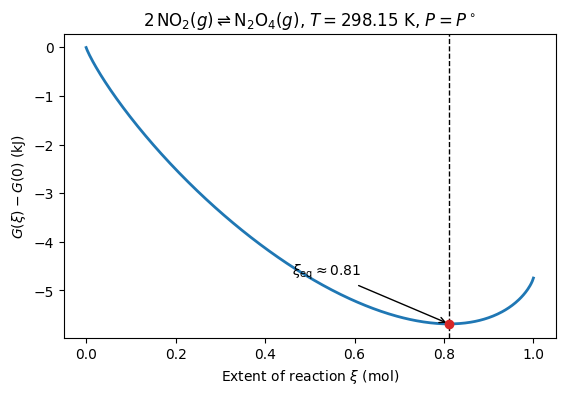
n N O 2 , e q ≈ 0.38 , n N 2 O 4 , e q ≈ 0.81. n_{\mathrm{NO_2},eq}\approx 0.38, \qquad n_{\mathrm{N_2O_4},eq}\approx 0.81. n N O 2 , e q ≈ 0.38 , n N 2 O 4 , e q ≈ 0.81. G ( ξ ) G(\xi) G ( ξ ) ξ e q \xi_{\mathrm{eq}} ξ eq ¶ The equilibrium condition Δ r G = 0 \Delta_r G = 0 Δ r G = 0 G ( ξ ) G(\xi) G ( ξ ) y i ( ξ ) y_i(\xi) y i ( ξ ) P = P ∘ P=P^\circ P = P ∘
G ( ξ ) − G ( 0 ) = ξ Δ r G ∘ + R T [ ( 2 − 2 ξ ) ln y N O 2 ( ξ ) + ξ ln y N 2 O 4 ( ξ ) ] . G(\xi) - G(0)
= \xi\,\Delta_r G^{\circ}
+ RT\!\left[(2-2\xi)\ln y_{\mathrm{NO_2}}(\xi) + \xi\ln y_{\mathrm{N_2O_4}}(\xi)\right]. G ( ξ ) − G ( 0 ) = ξ Δ r G ∘ + RT [ ( 2 − 2 ξ ) ln y N O 2 ( ξ ) + ξ ln y N 2 O 4 ( ξ ) ] . The first term is the “bookkeeping” shift in standard chemical potentials; the second is the ideal-mixing entropy that prevents the reaction from running to completion. Plotting:
import numpy as np
import matplotlib.pyplot as plt

R = 8.314462618          # J mol^-1 K^-1
T = 298.15
dG_std = -4.74e3         # J per mole of reaction
K_eq = np.exp(-dG_std / (R*T))

def G_of_xi(xi):
    n_NO2 = 2 - 2*xi
    n_N2O4 = xi
    n_tot = 2 - xi
    mix = 0.0
    if n_NO2 > 0:
        mix += n_NO2 * np.log(n_NO2 / n_tot)
    if n_N2O4 > 0:
        mix += n_N2O4 * np.log(n_N2O4 / n_tot)
    return xi*dG_std + R*T*mix   # J (per initial 2 mol NO2)

xis = np.linspace(1e-4, 1 - 1e-4, 400)
G_vals = np.array([G_of_xi(x) for x in xis]) / 1e3   # kJ

# Analytical xi_eq from K = xi(2-xi)/(2-2xi)^2
from scipy.optimize import brentq
xi_eq = brentq(lambda x: x*(2-x)/(2-2*x)**2 - K_eq, 0.01, 0.99)

fig, ax = plt.subplots(figsize=(6.0, 4.0))
ax.plot(xis, G_vals, lw=2)
ax.axvline(xi_eq, color="k", ls="--", lw=1)
ax.plot([xi_eq], [G_of_xi(xi_eq)/1e3], "o", color="tab:red", zorder=5)
ax.annotate(fr"$\xi_{{\mathrm{{eq}}}} \approx {xi_eq:.2f}$",
            xy=(xi_eq, G_of_xi(xi_eq)/1e3),
            xytext=(xi_eq - 0.35, G_of_xi(xi_eq)/1e3 + 1.0),
            arrowprops=dict(arrowstyle="->", lw=1))
ax.set_xlabel(r"Extent of reaction $\xi$ (mol)")
ax.set_ylabel(r"$G(\xi) - G(0)$ (kJ)")
ax.set_title(r"$2\,\mathrm{NO_2}(g) \rightleftharpoons \mathrm{N_2O_4}(g)$, "
             r"$T=298.15$ K, $P=P^\circ$")
fig.subplots_adjust(left=0.14, right=0.96, top=0.90, bottom=0.14)
plt.show()
The minimum of G ( ξ ) G(\xi) G ( ξ ) ξ e q \xi_{eq} ξ e q K K K Δ r G ∘ < 0 \Delta_r G^\circ < 0 Δ r G ∘ < 0 ξ \xi ξ R T ∑ n i ln y i RT\sum n_i \ln y_i RT ∑ n i ln y i N 2 O 4 \mathrm{N_2O_4} N 2 O 4 the reason chemical equilibrium is generically an interior minimum rather than either pure reactants or pure products.
Interactive visualization ¶ 7.1.5 Temperature dependence: the van’t Hoff equation ¶ The temperature dependence of K K K
( ∂ ∂ T Δ r G ∘ T ) P = − Δ r H ∘ T 2 . \left(\frac{\partial}{\partial T}\frac{\Delta_r G^{\circ}}{T}\right)_P
= -\frac{\Delta_r H^{\circ}}{T^2}. ( ∂ T ∂ T Δ r G ∘ ) P = − T 2 Δ r H ∘ . Using Δ r G ∘ = − R T ln K \Delta_r G^{\circ}=-RT\ln K Δ r G ∘ = − RT ln K van’t Hoff equation :
( ∂ ln K ∂ T ) P = Δ r H ∘ R T 2 . \boxed{
\left(\frac{\partial \ln K}{\partial T}\right)_P
= \frac{\Delta_r H^{\circ}}{RT^2}.
} ( ∂ T ∂ ln K ) P = R T 2 Δ r H ∘ . An equivalent integrated form between T 1 T_1 T 1 T 2 T_2 T 2 Δ r H ∘ \Delta_r H^{\circ} Δ r H ∘
ln [ K ( T 2 ) K ( T 1 ) ] = − Δ r H ∘ R ( 1 T 2 − 1 T 1 ) . \boxed{
\ln\!\left[\frac{K(T_2)}{K(T_1)}\right]
= -\frac{\Delta_r H^{\circ}}{R}\!\left(\frac{1}{T_2}-\frac{1}{T_1}\right).
} ln [ K ( T 1 ) K ( T 2 ) ] = − R Δ r H ∘ ( T 2 1 − T 1 1 ) . Example trend for 2 N O 2 ⇌ N 2 O 4 2\,\mathrm{NO_2}\rightleftharpoons\mathrm{N_2O_4} 2 N O 2 ⇌ N 2 O 4 ¶ At P = P ∘ P=P^{\circ} P = P ∘
T T T K K K ξ e q \xi_{eq} ξ e q 2 _2 2 250 205.18 0.97 298.15 6.74 0.81 350 0.17 0.23
Because Δ r H ∘ < 0 \Delta_r H^{\circ}<0 Δ r H ∘ < 0 K K K down and shifts equilibrium toward N O 2 \mathrm{NO_2} N O 2 N 2 O 4 \mathrm{N_2O_4} N 2 O 4
7.1.6 Computing K K K ¶ In § 7.1.3 we derived the key link between equilibrium and thermochemistry:
K ( T ) = exp ( − Δ r G ∘ ( T ) R T ) . K(T) = \exp\!\left(-\frac{\Delta_r G^{\circ}(T)}{RT}\right). K ( T ) = exp ( − RT Δ r G ∘ ( T ) ) . So if you can compute Δ r G ∘ \Delta_r G^{\circ} Δ r G ∘ getting Δ r G ∘ \Delta_r G^{\circ} Δ r G ∘
Step 0: Write the reaction (with phases) and choose a standard state ¶ Balance the reaction and include phases, e.g. N H 3 ( g ) \mathrm{NH_3(g)} N H 3 ( g ) N H 3 ( ℓ ) \mathrm{NH_3(\ell)} N H 3 ( ℓ )
Use a consistent standard state across all species (most modern tables use P ∘ = 1 b a r P^\circ=1\ \mathrm{bar} P ∘ = 1 bar T = 298.15 K T=298.15\ \mathrm{K} T = 298.15 K
Step 1: Pull species data at the same temperature ¶ For each species i i i
Option A (most common at 298.15 K): Δ f H i ∘ \Delta_f H_i^\circ Δ f H i ∘ S i ∘ S_i^\circ S i ∘ Δ f G i ∘ \Delta_f G_i^\circ Δ f G i ∘
Option B (temperature-dependent, e.g. T ≠ 298.15 K T\neq 298.15\,\mathrm{K} T = 298.15 K H i ∘ ( T ) H_i^\circ(T) H i ∘ ( T ) S i ∘ ( T ) S_i^\circ(T) S i ∘ ( T ) G i ∘ ( T ) G_i^\circ(T) G i ∘ ( T )
Where to get the data:
NIST Chemistry WebBook : fast way to grab Δ f H ∘ ( 298.15 K ) \Delta_f H^\circ(298.15\ \mathrm{K}) Δ f H ∘ ( 298.15 K ) S ∘ ( 298.15 K ) S^\circ(298.15\ \mathrm{K}) S ∘ ( 298.15 K )
NIST–JANAF Thermochemical Tables : best when you need H ∘ ( T ) H^\circ(T) H ∘ ( T ) S ∘ ( T ) S^\circ(T) S ∘ ( T )
ATcT (Active Thermochemical Tables) : best when you care about high-accuracy formation thermochemistry (often includes uncertainties). In practice, many workflows use ATcT for Δ f H ∘ \Delta_f H^\circ Δ f H ∘ and JANAF for S ∘ ( T ) S^\circ(T) S ∘ ( T ) .
Step 2: Convert species data into reaction values ¶ Once you have consistent species data, compute reaction properties using stoichiometric coefficients ν i \nu_i ν i
Δ r H ∘ = ∑ i ν i H i ∘ and Δ r S ∘ = ∑ i ν i S i ∘ . \Delta_r H^\circ = \sum_i \nu_i\,H_i^\circ
\qquad\text{and}\qquad
\Delta_r S^\circ = \sum_i \nu_i\,S_i^\circ. Δ r H ∘ = i ∑ ν i H i ∘ and Δ r S ∘ = i ∑ ν i S i ∘ . If your data are enthalpies of formation , this becomes the familiar “products minus reactants” form:
Δ r H ∘ = ∑ products ν p Δ f H p ∘ − ∑ reactants ν r Δ f H r ∘ . \Delta_r H^\circ
= \sum_{\text{products}} \nu_p\,\Delta_f H_p^\circ
-\sum_{\text{reactants}} \nu_r\,\Delta_f H_r^\circ. Δ r H ∘ = products ∑ ν p Δ f H p ∘ − reactants ∑ ν r Δ f H r ∘ . If an element appears in its standard state , then by convention Δ f H ∘ = 0 \Delta_f H^\circ = 0 Δ f H ∘ = 0 N 2 ( g ) \mathrm{N_2(g)} N 2 ( g ) H 2 ( g ) \mathrm{H_2(g)} H 2 ( g ) Δ r H ∘ \Delta_r H^\circ Δ r H ∘
Step 3: Compute Δ r G ∘ \Delta_r G^\circ Δ r G ∘ ¶ If you have Δ r H ∘ \Delta_r H^\circ Δ r H ∘ Δ r S ∘ \Delta_r S^\circ Δ r S ∘
Δ r G ∘ ( T ) = Δ r H ∘ ( T ) − T Δ r S ∘ ( T ) . \Delta_r G^\circ(T) = \Delta_r H^\circ(T) - T\,\Delta_r S^\circ(T). Δ r G ∘ ( T ) = Δ r H ∘ ( T ) − T Δ r S ∘ ( T ) . Step 4: Compute K K K ¶ Finally,
K ( T ) = exp ( − Δ r G ∘ ( T ) R T ) , log 10 K ( T ) = − Δ r G ∘ ( T ) ( ln 10 ) R T . K(T) = \exp\!\left(-\frac{\Delta_r G^\circ(T)}{RT}\right),
\qquad
\log_{10}K(T) = -\frac{\Delta_r G^\circ(T)}{(\ln 10)\,RT}. K ( T ) = exp ( − RT Δ r G ∘ ( T ) ) , log 10 K ( T ) = − ( ln 10 ) RT Δ r G ∘ ( T ) . For an ideal-gas reaction, this K K K ( P i / P ∘ ) (P_i/P^\circ) ( P i / P ∘ ) Q p Q_p Q p
For the Haber–Bosch reaction (as written in § 5.3),
N 2 ( g ) + 3 H 2 ( g ) → 2 N H 3 ( g ) . \mathrm{N_2(g) + 3H_2(g) \rightarrow 2NH_3(g)}. N 2 ( g ) + 3 H 2 ( g ) → 2N H 3 ( g ) . Using the reaction values quoted in § 5.3 at 298.15 K,
Δ r H ∘ ≈ − 92 k J m o l − 1 , Δ r S ∘ ≈ − 198 J m o l − 1 K − 1 , \Delta_r H^\circ \approx -92\ \mathrm{kJ\,mol^{-1}},\qquad
\Delta_r S^\circ \approx -198\ \mathrm{J\,mol^{-1}\,K^{-1}}, Δ r H ∘ ≈ − 92 kJ mo l − 1 , Δ r S ∘ ≈ − 198 J mo l − 1 K − 1 , gives
Δ r G ∘ ≈ − 92 k J m o l − 1 − ( 298.15 K ) ( − 0.198 k J m o l − 1 K − 1 ) ≈ − 33 k J m o l − 1 . \Delta_r G^\circ
\approx -92\ \mathrm{kJ\,mol^{-1}}
- (298.15\ \mathrm{K})\!\left(-0.198\ \mathrm{kJ\,mol^{-1}\,K^{-1}}\right)
\approx -33\ \mathrm{kJ\,mol^{-1}}. Δ r G ∘ ≈ − 92 kJ mo l − 1 − ( 298.15 K ) ( − 0.198 kJ mo l − 1 K − 1 ) ≈ − 33 kJ mo l − 1 . Then
K ( 298.15 K ) = exp ( − − 33 , 000 ( 8.314 ) ( 298.15 ) ) ≈ 6 × 1 0 5 . K(298.15\ \mathrm{K}) = \exp\!\left(-\frac{-33{,}000}{(8.314)(298.15)}\right)
\approx 6\times 10^{5}. K ( 298.15 K ) = exp ( − ( 8.314 ) ( 298.15 ) − 33 , 000 ) ≈ 6 × 1 0 5 . Interpretation. K ≫ 1 K\gg 1 K ≫ 1 N H 3 \mathrm{NH_3} N H 3 at the standard state . (Section 5.3 explains why temperature and pressure “knobs” still matter for industrial operation, where the 500 °C kinetic sweet spot drives K K K
Common pitfalls (and quick fixes) ¶ Wrong phase: H 2 O ( ℓ ) \mathrm{H_2O(\ell)} H 2 O ( ℓ ) H 2 O ( g ) \mathrm{H_2O(g)} H 2 O ( g ) N H 3 ( ℓ ) \mathrm{NH_3(\ell)} N H 3 ( ℓ ) N H 3 ( g ) \mathrm{NH_3(g)} N H 3 ( g ) S ∘ S^\circ S ∘ Δ f H ∘ \Delta_f H^\circ Δ f H ∘
Mixed standard states: make sure all species use the same P ∘ P^\circ P ∘
Unit mismatches: always reconcile kJ vs J and “per mole of reaction” vs “per mole of species.”
Sign mistakes: products minus reactants (or use ν i \nu_i ν i
Concept Checks ¶ Why is Δ r G = 0 \Delta_r G=0 Δ r G = 0 T , P T,P T , P T , V T,V T , V T , V T,V T , V
Why must Q p Q_p Q p K K K P ∘ P^\circ P ∘
How does comparing Q p Q_p Q p K K K
Inspecting Eq. (32) G ( ξ ) G(\xi) G ( ξ ) Δ r G ∘ ≪ 0 \Delta_r G^\circ \ll 0 Δ r G ∘ ≪ 0
What changes in the derivation of Δ r G = Δ r G ∘ + R T ln Q p \Delta_r G = \Delta_r G^\circ + RT\ln Q_p Δ r G = Δ r G ∘ + RT ln Q p
Key Takeaways ¶ Extent of reaction ξ \xi ξ d n i = ν i d ξ dn_i = \nu_i\,d\xi d n i = ν i d ξ
At constant T , P T,P T , P G G G Δ r G = ∑ i ν i μ i = 0 \Delta_r G = \sum_i\nu_i\mu_i = 0 Δ r G = ∑ i ν i μ i = 0
For ideal gases, Δ r G = Δ r G ∘ + R T ln Q p \Delta_r G = \Delta_r G^\circ + RT\ln Q_p Δ r G = Δ r G ∘ + RT ln Q p Δ r G ∘ = − R T ln K \Delta_r G^\circ = -RT\ln K Δ r G ∘ = − RT ln K
The sign of Δ r G \Delta_r G Δ r G Q p Q_p Q p K K K
The temperature dependence of K K K ∂ ln K / ∂ T = Δ r H ∘ / ( R T 2 ) \partial\ln K/\partial T = \Delta_r H^\circ/(RT^2) ∂ ln K / ∂ T = Δ r H ∘ / ( R T 2 )
Thermochemical tables (NIST WebBook, JANAF, ATcT) provide the Δ f H ∘ \Delta_f H^\circ Δ f H ∘ S ∘ S^\circ S ∘ Δ r G ∘ \Delta_r G^\circ Δ r G ∘ K K K