4.1. Entropy

Course-wide Conventions & Notation

Overview and Learning Objectives¶

Entropy completes the thermodynamic description of spontaneity by accounting for the dispersal of energy and matter. This section motivates entropy through examples where enthalpy alone fails, defines entropy as a state function via reversible heat, and derives the fundamental relation $dU=T\,dS-P\,dV$ for simple compressible systems.

In Chapter 3, we established the First Law toolkit: internal energy $U$, enthalpy $H$, heat capacities $C_V$ and $C_P$, and the five-step workflow for computing $q$, $w$, and $\Delta U$ under various process constraints. That toolkit tells us how much energy is exchanged — but not which direction a process will spontaneously proceed. We will see that exothermicity ($\Delta H < 0$) often favors spontaneity but does not fully determine it. The missing piece is entropy, a state function that provides crucial insight into the direction of spontaneous change.

In Chapter 2, we built a statistical-mechanical framework in which macroscopic properties emerge as ensemble averages over microstates. Entropy turns out to have a particularly natural microscopic interpretation: it measures how many microstates are consistent with a given macrostate. This section introduces entropy from the macroscopic side; Section 4.3 will close the loop by connecting entropy to the partition function $Q$.

Learning objectives:

• Explain why exothermicity ($\Delta H<0$) does not by itself guarantee spontaneity.

• Define entropy $S$ as a state function using $dS=\delta q_{\mathrm{rev}}/T$.

• Verify that $\delta q_{\mathrm{rev}}/T$ is exact for an ideal gas by applying the cross-derivative test.

• Use the First Law for a reversible $PV$-only process to derive $dU=T\,dS-P\,dV$.

• Compute entropy changes by integrating $\delta q_{\mathrm{rev}}/T$ along a convenient reversible path, including for irreversible processes.

Core Ideas and Derivations¶

Exothermicity and Spontaneity¶

Exothermic reactions are often — but not always — spontaneous. An exothermic process releases heat to its surroundings, corresponding to a negative enthalpy change, $\Delta H < 0$. While this heat release can drive a process forward, enthalpy alone does not guarantee spontaneity; we must also consider entropy.

An Example: Formation of Liquid Water¶

Consider the formation of two moles of liquid water from hydrogen and oxygen gases at 298.15 K and 1 bar:

The standard enthalpy change for this reaction is -571.66 kJ for two moles of H$_2$O(l), indicating an exothermic process. The reaction releases heat:

It is fortunate that water formation is exothermic, as this makes the reaction more likely to proceed spontaneously under standard conditions.

A Counter Example: Mixing of Two Ideal Gases¶

If we mix two ideal gases, such as Ar and Kr, their intermolecular interactions are negligible (ideal-gas behavior), so $\Delta H = 0$. Nonetheless, mixing occurs spontaneously once the partition is removed.

Source

import numpy as np
import matplotlib.pyplot as plt
from scipy.constants import k, eV
from labellines import labelLines
from myst_nb import glue

rng = np.random.default_rng(8251991)

fig, axs = plt.subplot_mosaic([[0, 1]], figsize=(8, 4), constrained_layout=True, sharex=True, sharey=True)

# Before
axs[0].set_title('Before Opening the Stopper')
x_Ar = rng.uniform(-4, 4, 6)
y_Ar = rng.uniform(2, 5, 6)
axs[0].scatter(x_Ar, y_Ar, color='r', label='Ar', s=100)

x_Kr = rng.uniform(-4, 4, 6)
y_Kr = rng.uniform(-5, -2, 6)
axs[0].scatter(x_Kr, y_Kr, color='b', label='Kr', s=100)

# Ar region
axs[0].plot([1, 1], [0, 1], color='k')
axs[0].plot([1, 5], [1, 1], color='k')
axs[0].plot([5, 5], [1, 6], color='k')
axs[0].plot([5, -5], [6, 6], color='k')
axs[0].plot([-5, -5], [6, 1], color='k')
axs[0].plot([-5, -1], [1, 1], color='k')
axs[0].plot([-1, -1], [1, 0], color='k')

# Kr region
axs[0].plot([1, 1], [0, -1], color='k')
axs[0].plot([1, 5], [-1, -1], color='k')
axs[0].plot([5, 5], [-1, -6], color='k')
axs[0].plot([5, -5], [-6, -6], color='k')
axs[0].plot([-5, -5], [-6, -1], color='k')
axs[0].plot([-5, -1], [-1, -1], color='k')
axs[0].plot([-1, -1], [-1, 0], color='k')

# Closed stopper
axs[0].plot([-1.5, 1.5], [0, 0], color='m', lw=2)
axs[0].text(2, 0, "Stopper (closed)", fontsize=10, ha='left', va='center', color='m')
axs[0].set_aspect('equal')
axs[0].axis('off')

# After
axs[1].set_title('After Opening the Stopper')
x_Ar = rng.uniform(-4, 4, 6)
y_Ar_1 = rng.uniform(2, 5, 3)
y_Ar_2 = rng.uniform(-5, -2, 3)
y_Ar = np.concatenate((y_Ar_1, y_Ar_2))
axs[1].scatter(x_Ar, y_Ar, color='r', label='Ar', s=100)

x_Kr = rng.uniform(-4, 4, 6)
y_Kr_1 = rng.uniform(2, 5, 3)
y_Kr_2 = rng.uniform(-5, -2, 3)
y_Kr = np.concatenate((y_Kr_1, y_Kr_2))
axs[1].scatter(x_Kr, y_Kr, color='b', label='Kr', s=100)

axs[1].plot([1, 1], [0, 1], color='k')
axs[1].plot([1, 5], [1, 1], color='k')
axs[1].plot([5, 5], [1, 6], color='k')
axs[1].plot([5, -5], [6, 6], color='k')
axs[1].plot([-5, -5], [6, 1], color='k')
axs[1].plot([-5, -1], [1, 1], color='k')
axs[1].plot([-1, -1], [1, 0], color='k')
axs[1].plot([1, 1], [0, -1], color='k')
axs[1].plot([1, 5], [-1, -1], color='k')
axs[1].plot([5, 5], [-1, -6], color='k')
axs[1].plot([5, -5], [-6, -6], color='k')
axs[1].plot([-5, -5], [-6, -1], color='k')
axs[1].plot([-5, -1], [-1, -1], color='k')
axs[1].plot([-1, -1], [-1, 0], color='k')

# Open stopper
axs[1].plot([-5, -2], [0, 0], color='m', lw=2)
axs[1].text(2, 0, "Stopper (open)", fontsize=10, ha='left', va='center', color='m')
axs[1].axis('off')
axs[1].set_aspect('equal')
axs[1].legend(bbox_to_anchor=(1.05, 1), loc='upper left', borderaxespad=0.)

fig.suptitle(r'$\Delta H = 0$')

plt.show()
plt.close(fig)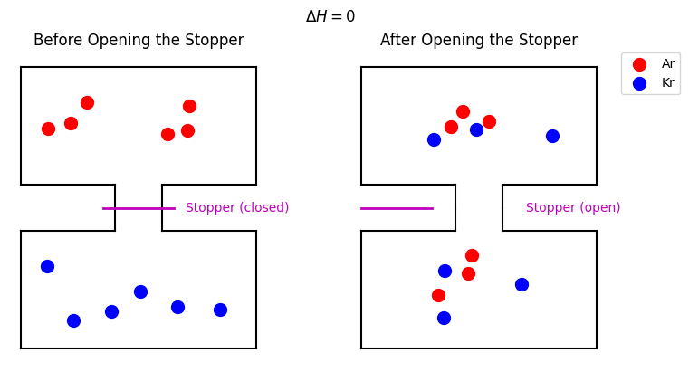

Mixing of two ideal gases before and after opening the stopper that separates them.

Even though $\Delta H = 0$, the process is still spontaneous. If you were shown the “before” and “after” snapshots without additional labels, you would know the natural direction of mixing. This spontaneous behavior underscores that enthalpy alone cannot capture whether a process will occur without additional driving forces. That driving force is entropy — and we can already anticipate why. From each gas’s perspective, removing the partition is equivalent to a free expansion: the volume accessible to each gas doubles. As we will show below, doubling the available volume at constant temperature increases the entropy by $nR\ln 2$ per component. For a symmetric mixture of $n$ moles each of Ar and Kr,

The entropy of the mixed state exceeds that of the separated state, so mixing is the spontaneous direction. (We will derive the result $\Delta S = nR\ln(V_2/V_1)$ in full below; we quote it here to motivate what follows.)

Definition of Entropy¶

The General Claim¶

In Section 3.1, we noted a key distinction: $dU$ is an exact differential, while $\delta q$ and $\delta w$ are inexact — their values depend on the path. We also foreshadowed that “dividing the inexact differential $\delta q$ by $T$ produces the exact differential $dS$.”

It can be shown — via the Clausius theorem (a consequence of the second law) or by identifying $1/T$ as an integrating factor (Appendix A) — that $\delta q_{\mathrm{rev}}/T$ is always an exact differential, regardless of the substance. We therefore define entropy through

The change in entropy between two states $A$ and $B$ is

Because $dS$ is exact, $\Delta S$ depends only on the initial and final states — not on the path. However, computing $\Delta S$ requires evaluating the integral along a reversible path (since $dS = \delta q_{\mathrm{rev}}/T$ holds only for reversible processes). For an irreversible process between the same two states, we construct any convenient reversible path connecting them and integrate along that path instead.

Verification: Ideal Gas¶

Rather than proving the general result, let us verify that $\delta q_{\mathrm{rev}}/T$ is exact for an ideal gas — a case where we can check directly.

From Section 3.2, the First Law for a reversible process with only $PV$ work, using $V$ and $T$ as independent variables, gives

For any ideal gas (not just monatomic), $(\partial U/\partial V)_T = 0$ and $P = Nk_{\mathrm{B}}T/V$, so

This is inexact: the cross-derivative test gives $(\partial C_V/\partial V)_T = 0$ but $\partial(Nk_{\mathrm{B}}T/V)/\partial T\big|_V = Nk_{\mathrm{B}}/V \neq 0$.

Now divide by $T$:

Apply the cross-derivative test to $M(T,V) = C_V/T$ and $N(T,V) = Nk_{\mathrm{B}}/V$:

Both mixed partials are zero, so they are equal: $\delta q_{\mathrm{rev}}/T$ is exact. Dividing by $T$ converted an inexact differential into an exact one, confirming the entropy definition for this case.

Fundamental Thermodynamic Relation¶

From the definition of entropy, $\delta q_{\text{rev}} = T\,dS$. For a simple closed system with only $PV$ work ($\delta w_{\mathrm{rev}} = -P\,dV$), the First Law gives

This is the fundamental thermodynamic relation for a simple compressible system:

Notice what has happened: the First Law in the form $dU = \delta q + \delta w$ involves two inexact differentials that combine to give one exact differential. The fundamental relation rewrites the same physics using three exact differentials — $dU$, $dS$, and $dV$. The path-dependent $\delta q_{\mathrm{rev}}$ has been replaced by the state-function product $T\,dS$, and the path-dependent $\delta w_{\mathrm{rev}}$ by $-P\,dV$. Converting inexact differentials into exact ones is the central mathematical achievement of introducing entropy.

Here, $U$ is naturally expressed as a function of the extensive variables $S$ and $V$. In systems with additional types of work (e.g., electrical, surface, magnetic), the more general relation becomes

Worked Examples¶

Example 1: Isothermal expansion (reversible)¶

Problem. Compute $\Delta S$ when one mole of an ideal gas expands reversibly and isothermally from $V_1$ to $V_2 = 2V_1$.

Solution. For a reversible isothermal expansion of an ideal gas,

Along a reversible isotherm of an ideal gas, $dU = 0$ (since $U$ depends only on $T$), so $\delta q_{\mathrm{rev}} = -\delta w_{\mathrm{rev}} = P\,dV = nRT\,dV/V$. Therefore

With $n = 1\ \mathrm{mol}$ and $V_2 = 2V_1$:

Result. Doubling the volume reversibly at constant $T$ increases the entropy by $R\ln 2$ per mole. This is the result we quoted earlier when computing $\Delta S_{\mathrm{mix}}$ for ideal-gas mixing.

Example 2: Free expansion (irreversible)¶

Problem. Compute $\Delta S$ when one mole of an ideal gas undergoes free expansion from $V_1$ to $V_2 = 2V_1$ inside a rigid, insulated container (as in the Section 3.1 worked example).

Solution. In the free expansion, $P_{\mathrm{ext}} = 0$, so $w = 0$. The container is insulated, so $q = 0$. By the First Law, $\Delta U = 0$, which means $\Delta T = 0$ for an ideal gas.

But $q = 0$ does not mean $\Delta S = 0$! The definition $dS = \delta q_{\mathrm{rev}}/T$ applies to a reversible path, and free expansion is decidedly irreversible. To compute $\Delta S$, we need a reversible path connecting the same initial and final states.

The initial and final states have the same $T$ but different $V$ — exactly the endpoints of Example 1. Since $S$ is a state function,

Result. The entropy change is the same as for the reversible isothermal expansion — because entropy is a state function. What differs between the two processes is the entropy of the surroundings: in the reversible case, $\Delta S_{\mathrm{surr}} = -R\ln 2$ (the reservoir loses heat $q_{\mathrm{rev}}$ at temperature $T$), so $\Delta S_{\mathrm{total}} = 0$. In the free expansion, $\Delta S_{\mathrm{surr}} = 0$ (no heat exchanged), so $\Delta S_{\mathrm{total}} = R\ln 2 > 0$ — entropy was produced by the irreversible process.

Concept Checks¶

1. In the ideal-gas mixing example, why can $\Delta H = 0$ but the process still be spontaneous?

2. Why must $\Delta S$ be computed along a reversible path even for an irreversible process between the same states?

3. What are the natural variables of $U$ for a simple compressible system, and how do they appear in $dU$?

4. How does the sign of $\Delta S_{\mathrm{total}}$ (system + surroundings) relate to “directionality” (arrow of time) in spontaneous processes?

5. Two ideal-gas processes connect the same initial and final states: one reversible, one irreversible. Compare $\Delta S_{\mathrm{system}}$, $\Delta S_{\mathrm{surroundings}}$, and $\Delta S_{\mathrm{total}}$ for the two processes.

Key Takeaways¶

• Spontaneity depends on more than enthalpy; entropy accounts for dispersal and multiplicity of accessible states.

• Entropy is defined by $dS = \delta q_{\mathrm{rev}}/T$ and is a state function: its value depends only on the state, not the path.

• Dividing $\delta q_{\mathrm{rev}}$ by $T$ converts an inexact differential into an exact one — this is the central mathematical role of entropy.

• For reversible $PV$-only processes, $dU = T\,dS - P\,dV$ is the fundamental thermodynamic relation, expressing the First Law entirely in terms of exact differentials.

• Entropy changes for irreversible processes are computed by finding a convenient reversible path between the same initial and final states and integrating $\delta q_{\mathrm{rev}}/T$ along that path.