4.2. Carnot Cycle - Physical Chemistry II

Overview and Learning Objectives¶

The Carnot cycle is a fully reversible heat-engine cycle that sets the maximum efficiency any engine can achieve between two reservoir temperatures. Using the entropy definition $dS=\delta q_{\mathrm{rev}}/T$ , the cycle relates heat flows to temperature and establishes $\eta_{\mathrm{Carnot}}=1-T_{\mathrm{cold}}/T_{\mathrm{hot}}$ . The same reasoning yields a second-law statement about the direction of spontaneous heat flow.

This section connects entropy to the performance limits of heat engines using the Carnot cycle. It develops four linked ideas:

Entropy and reversible heat. From Section 4.1, the differential definition of entropy for a reversible path is
$dS = \frac{\delta q_{\mathrm{rev}}}{T}.$
(1)
Entropy change tracks how much reversible heat flows at a given temperature.
The Carnot cycle as a “best possible” engine. A Carnot engine is an idealized, fully reversible cycle operating between two thermal reservoirs: a hot reservoir at temperature $T_{\mathrm{hot}}$ and a cold reservoir at $T_{\mathrm{cold}}$ . The cycle consists of two reversible isotherms and two reversible adiabats.
Maximum efficiency for converting heat to work. For any engine operating between the same two reservoir temperatures, the Carnot engine has the maximum possible efficiency:
$\eta_{\mathrm{Carnot}} = 1 - \frac{T_{\mathrm{cold}}}{T_{\mathrm{hot}}}.$
(2)
Second law as the direction of heat flow. A two-body argument shows that spontaneous heat flow must go from higher temperature to lower temperature, because the total entropy of an isolated system must not decrease.

Throughout, we use the standard Carnot labeling $A \to B \to C \to D \to A$ :

$A\to B$ : isothermal expansion at $T_{\mathrm{hot}}$
$B\to C$ : adiabatic expansion (insulated)
$C\to D$ : isothermal compression at $T_{\mathrm{cold}}$
$D\to A$ : adiabatic compression (insulated)

Learning objectives:

Describe the four reversible steps of the Carnot cycle (two isotherms and two adiabats) on a $P$ – $V$ diagram.
Use entropy changes on reversible isotherms and adiabats to show $\Delta S_{\mathrm{cycle}}=0$ .
Derive the Carnot efficiency $\eta_{\mathrm{Carnot}}=1-T_{\mathrm{cold}}/T_{\mathrm{hot}}$ .
Explain why spontaneous heat flow from hot to cold is required by non-decreasing total entropy.

Core Ideas and Derivations¶

The Cycle¶

The figure below plots the Carnot cycle on a pressure–volume (P–V) diagram for an ideal gas. The key geometric features are:

The isotherms (red/blue) follow the ideal-gas relation $P = nRT/V$ at fixed temperature.
The adiabats (dashed/dotted) are steeper than the isotherms and follow $PV^\gamma = \text{constant}$ for a reversible adiabatic process of an ideal gas (Section 3.2).

import numpy as np
import matplotlib.cm as cm
import matplotlib.pyplot as plt
from scipy.constants import R as R_J_per_K_mol
from labellines import labelLines
from myst_nb import glue

# Constants
R = R_J_per_K_mol / 1000  # J/K/mol to kJ/K/mol (keeps PV values numerically small for plotting)

# Isothermal Process for Ideal Gas
def P_isothermal_ideal_gas(V, T, n):
    return n * R * T / V

# Adiabatic Process for Ideal Gas
def P_adiabatic_ideal_gas(V, V1, P1, gamma=5/3):
    return P1 * (V1 / V) ** gamma

# Intersection of two pressure curves
def intersection(P1, P2, V):
    return V[np.argmin(np.abs(P1 - P2))]

# Plotting the Carnot Cycle
fig, axs = plt.subplots(1, 1, figsize=(4, 4))

# Calculate the pressure for each segment of the cycle
V = np.linspace(0.1, 5, 1000)  # L
T_hot = 298.15  # K
T_cold = 273.15  # K
n = 1  # mol
V_A = 0.5  # L
V_C = 1.0  # L
P_AB = P_isothermal_ideal_gas(V, T_hot, n)
P_DA = P_adiabatic_ideal_gas(V, V_A, P_isothermal_ideal_gas(V_A, T_hot, n))
P_CD = P_isothermal_ideal_gas(V, T_cold, n)
P_BC = P_adiabatic_ideal_gas(V, V_C, P_isothermal_ideal_gas(V_C, T_cold, n))

# Plot the segments
isotherm_1 = axs.plot(V, P_AB, "r-", label=r'A$\rightarrow$B isothermal expansion ($T_{\text{hot}}$)')
adiabat_1 = axs.plot(V, P_BC, "k:", label=r'B$\rightarrow$C adiabatic expansion', zorder=-10)
isotherm_2 = axs.plot(V, P_CD, "b-", label=r'C$\rightarrow$D isothermal compression ($T_{\text{cold}}$)')
adiabat_2 = axs.plot(V, P_DA, "k--", label=r'D$\rightarrow$A adiabatic compression', zorder=-10)

# Legend
axs.legend(bbox_to_anchor=(1.05, 1), loc='upper left', borderaxespad=0., title="Steps")

# Mark the points
axs.plot(V_A, P_isothermal_ideal_gas(V_A, T_hot, n), "ks", markerfacecolor='none')
axs.annotate("A", (V_A, P_isothermal_ideal_gas(V_A, T_hot, n)), textcoords="offset points", xytext=(10, 10), ha='center', va='center')
V_B = intersection(P_AB, P_BC, V)
P_B = P_isothermal_ideal_gas(V_B, T_hot, n)
axs.plot(V_B, P_B, "ks", markerfacecolor='none')
axs.annotate("B", (V_B, P_B), textcoords="offset points", xytext=(10, 10), ha='center', va='center')
V_C = intersection(P_BC, P_CD, V)
P_C = P_isothermal_ideal_gas(V_C, T_cold, n)
axs.plot(V_C, P_C, "ks", markerfacecolor='none')
axs.annotate("C", (V_C, P_C), textcoords="offset points", xytext=(-10, -10), ha='center', va='center')
V_D = intersection(P_CD, P_DA, V)
P_D = P_isothermal_ideal_gas(V_D, T_cold, n)
axs.plot(V_D, P_D, "ks", markerfacecolor='none')
axs.annotate("D", (V_D, P_D), textcoords="offset points", xytext=(-10, -10), ha='center', va='center')

axs.set_xlim(0.4, 1.1)
axs.set_ylim(2, 6)

axs.set_xticks([V_A, V_B, V_C, V_D])
axs.set_xticklabels([r"$V_A$", r"$V_B$", r"$V_C$", r"$V_D$"])

P_A = P_isothermal_ideal_gas(V_A, T_hot, n)
axs.set_yticks([P_A, P_B, P_C, P_D])
axs.set_yticklabels([r"$P_A$", r"$P_B$", r"$P_C$", r"$P_D$"])

# Add heat-flow annotations (matches the lecture sketch: heat in on the hot isotherm, heat out on the cold isotherm)
x = (V_B + V_D) / 2
y = (P_B + P_D) / 2
axs.annotate("system\nabsorbs\nheat", (x, y - 0.1), textcoords="offset points", xytext=(50, 50), ha='center', va='center', fontsize=10, color='r', arrowprops=dict(facecolor='r', shrink=0.05, edgecolor='w', width=2, headwidth=8, headlength=8))
axs.annotate("system\nreleases\nheat", (x, y - 0.1), textcoords="offset points", xytext=(-50, -50), ha='center', va='center', fontsize=10, color='b', arrowprops=dict(facecolor='b', shrink=0.05, edgecolor='w', width=2, headwidth=8, headlength=8))

axs.grid()

plt.show()
plt.close(fig)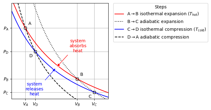

The Carnot cycle for an ideal gas. The isothermal expansion and compression curves follow the ideal-gas equation (Boyle’s-law form at fixed $T$ ), while the adiabatic expansion and compression curves follow the adiabatic equation (which produces a steeper curve than the isotherms).

Step-by-step thermodynamic description¶

Step	Process type	Thermal contact	Heat $q$	Entropy change $\Delta S$	Qualitative work
$A\to B$	Reversible isothermal expansion at $T_{\mathrm{hot}}$	Hot reservoir	$q_{AB} > 0$	$\Delta S_{AB} = q_{AB}/T_{\mathrm{hot}}$	System does work on surroundings ( $w_{AB} < 0$ )
$B\to C$	Reversible adiabatic expansion	Insulated	$q_{BC}=0$	$\Delta S_{BC}=0$	System does work; temperature drops ( $w_{BC} < 0$ )
$C\to D$	Reversible isothermal compression at $T_{\mathrm{cold}}$	Cold reservoir	$q_{CD} < 0$	$\Delta S_{CD} = q_{CD}/T_{\mathrm{cold}}$	Surroundings do work on system ( $w_{CD} > 0$ )
$D\to A$	Reversible adiabatic compression	Insulated	$q_{DA}=0$	$\Delta S_{DA}=0$	Surroundings do work on system; $T$ rises ( $w_{DA} > 0$ )

Two quick consequences:

Because adiabatic steps have $q=0$ , the reversible definition $dS = \delta q_{\mathrm{rev}}/T$ gives $\Delta S = 0$ on the adiabats (entropy is constant on a reversible adiabat — such a process is called isentropic).
Over one full cycle, the system returns to its initial state, so
$\Delta S_{\text{cycle}} = \Delta S_{AB} + \Delta S_{BC} + \Delta S_{CD} + \Delta S_{DA} = \Delta S_{AB} + \Delta S_{CD} = 0,$
(3)
which is exactly the relation we should expect: $S$ is a state function, so its change over any closed cycle must vanish.

How to Operate a Carnot Cycle/Engine¶

The Carnot cycle can be realized conceptually with a gas-filled cylinder, a piston loaded with weights, and two thermal reservoirs. The core idea: you alternate between (i) placing the gas in contact with a thermal reservoir so it can exchange heat reversibly at a fixed temperature (isotherms), and (ii) insulating the gas so it cannot exchange heat (adiabats).

$A\to B$ : isothermal expansion at $T_{\mathrm{hot}}$ Put the cylinder in contact with the hot thermal source. Remove weights slowly so the piston rises quasi-statically. The system absorbs heat $q_{AB}$ from the hot reservoir to keep $T$ constant, while doing work on the weights.
$B\to C$ : adiabatic expansion (insulated) Remove the thermal contact and insulate the cylinder. Continue removing weights slowly so the piston rises. No heat flows ( $q=0$ ), so the work done by the gas comes from its internal energy, and the temperature drops from $T_{\mathrm{hot}}$ to $T_{\mathrm{cold}}$ .
$C\to D$ : isothermal compression at $T_{\mathrm{cold}}$ Put the cylinder in contact with the cold thermal source. Add weights slowly so the piston lowers. The surroundings do work on the gas, and the gas releases heat $q_{CD}$ to the cold reservoir to keep $T$ constant.
$D\to A$ : adiabatic compression (insulated) Insulate the cylinder again and keep adding weights slowly to compress the gas. With no heat exchange, the work done on the gas increases its internal energy and raises the temperature back to $T_{\mathrm{hot}}$ , returning to state $A$ .

The schematic below illustrates each step, showing the thermal contact, piston position, and energy flows at the end of each process.

import numpy as np
import matplotlib.cm as cm
import matplotlib.pyplot as plt
from scipy.constants import R as R_J_per_K_mol
from labellines import labelLines
from myst_nb import glue

fig, axs = plt.subplot_mosaic([[0, 1, 2, 3]], figsize=(8, 4), constrained_layout=True, sharex=True, sharey=True)

# Each panel shows the END state of the corresponding step.
# Step 1: A→B (isothermal expansion at T_hot) → ends at state B
# Step 2: B→C (adiabatic expansion)            → ends at state C
# Step 3: C→D (isothermal compression at T_cold) → ends at state D
# Step 4: D→A (adiabatic compression)          → ends at state A

titles = [
    r'Step 1: A$\to$B',
    r'Step 2: B$\to$C',
    r'Step 3: C$\to$D',
    r'Step 4: D$\to$A',
]
# Piston heights at the END state of each step (B, C, D, A)
piston_height = [3.5, 4.5, 2.5, 1.5]
# State labels at the END of each step
end_state = ["B", "C", "D", "A"]
# Thermal contact during each step
thermal_label = [r'$T_{\text{hot}}$', 'insulation', r'$T_{\text{cold}}$', 'insulation']

for i in range(4):
    axs[i].set_title(titles[i], fontsize=10)

    # Cylinder
    axs[i].plot([0, 0], [5, 0], 'k-')
    cylinder = axs[i].plot([0, 3], [0, 0], 'k-', label='cylinder')
    axs[i].plot([3, 3], [0, 5], 'k-')
    labelLines(cylinder, xvals=[1.5], fontsize=10, color='k')

    # Thermal source / insulation block
    axs[i].plot([0, 0], [-1, -2], 'k:')
    thermal_source = axs[i].plot([0, 3], [-2, -2], 'k:', label='thermal source')
    axs[i].plot([3, 3], [-2, -1], 'k:')
    axs[i].plot([3, 0], [-1, -1], 'k:')
    labelLines(thermal_source, xvals=[1.5], fontsize=10, color='k')
    axs[i].text(1.5, -1.5, thermal_label[i], fontsize=10, ha='center', va='center')

    # Piston
    axs[i].plot([1.5, 1.5], [piston_height[i], 6], 'k-', lw=2)
    piston = axs[i].plot([0, 3], [piston_height[i], piston_height[i]], 'k-', lw=2, label='piston')
    labelLines(piston, xvals=[1.5], fontsize=10, color='k')

    # P, V labels at end state
    label = '$V_{\\text{' + end_state[i] + '}}, P_{\\text{' + end_state[i] + '}}$'
    axs[i].text(1.5, 0.75, label, fontsize=10, ha='center', va='center')

    # Heat transfer annotations (only on isothermal steps)
    if i == 0:  # A→B: system absorbs heat from hot reservoir
        axs[i].annotate("heat in", (0.5, 0.75), textcoords="offset points", xytext=(0, -60), ha='center', va='center', fontsize=10, color='r', arrowprops=dict(facecolor='r', shrink=0.05, edgecolor='w', width=2, headwidth=8, headlength=8))
    if i == 2:  # C→D: system releases heat to cold reservoir
        axs[i].annotate("heat out", (0.5, -1.5), textcoords="offset points", xytext=(0, 60), ha='center', va='center', fontsize=10, color='r', arrowprops=dict(facecolor='r', shrink=0.05, edgecolor='w', width=2, headwidth=8, headlength=8))

    # Work annotations (only on the two most illustrative steps)
    if i == 0:  # A→B: expansion, system does work
        axs[i].annotate("work done by system", (1.5, piston_height[i] - 0.1), textcoords="offset points", xytext=(0, -30), ha='center', va='center', fontsize=10, color='b', arrowprops=dict(facecolor='b', shrink=0.05, edgecolor='w', width=2, headwidth=8, headlength=8))
    if i == 2:  # C→D: compression, surroundings do work
        axs[i].annotate("work done on system", (1.5, piston_height[i] - 1.5), textcoords="offset points", xytext=(0, 30), ha='center', va='center', fontsize=10, color='b', arrowprops=dict(facecolor='b', shrink=0.05, edgecolor='w', width=2, headwidth=8, headlength=8))

    # Axis settings
    axs[i].set_ylim(-3, 6)

plt.show()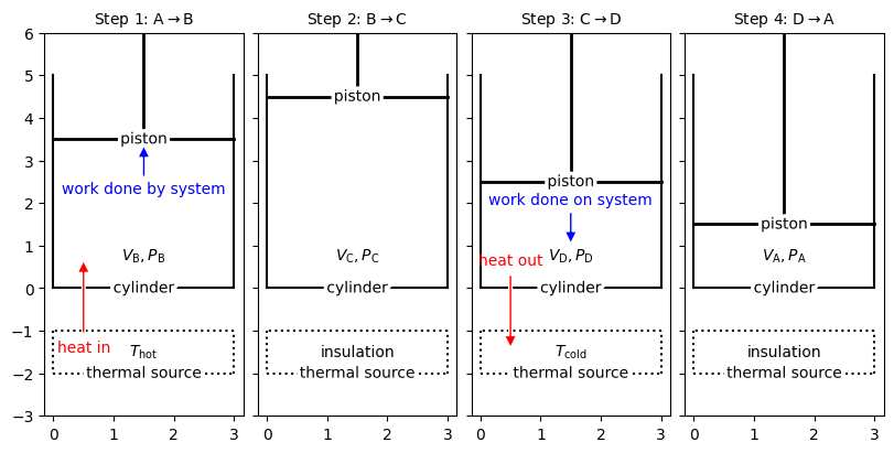

Schematic of the four Carnot-cycle steps. Each panel shows the thermal contact during that step and the piston position at its endpoint. Heat exchange occurs only during the isothermal steps (Steps 1 and 3); the adiabatic steps (Steps 2 and 4) are insulated.

Maximum Efficiency of Converting Heat to Work (Carnot Efficiency)¶

We define the heat quantities on the two isothermal legs from the system’s perspective, following the course sign convention ( $q > 0$ when heat is absorbed by the system):

$q_{AB} > 0$ : heat absorbed by the system from the hot reservoir during step $A \to B$
$q_{CD} < 0$ : heat released by the system to the cold reservoir during step $C \to D$

For one complete cycle, $\Delta U_{\mathrm{cycle}} = 0$ (state function returns to its initial value), so the First Law gives

0 = (q_{AB} + q_{CD}) + w_{\mathrm{cycle}},

(4)

where $w_{\mathrm{cycle}}$ is the total work over the cycle in the course convention ( $w > 0$ when work is done on the system). Since the engine does net work on the surroundings, $w_{\mathrm{cycle}} < 0$ , and the net work output is

W_{\mathrm{out}} \equiv -w_{\mathrm{cycle}} = q_{AB} + q_{CD}.

(5)

The thermal efficiency is defined as the fraction of absorbed heat converted to useful work output:

\eta = \frac{W_{\mathrm{out}}}{q_{AB}} = \frac{q_{AB} + q_{CD}}{q_{AB}}.

(6)

Now use the entropy definition on the isotherms:

\Delta S_{AB} = \frac{q_{AB}}{T_{\mathrm{hot}}},\qquad \Delta S_{CD} = \frac{q_{CD}}{T_{\mathrm{cold}}}.

(7)

Because the full reversible cycle returns the system to its initial state,

\Delta S_{\text{cycle}} = \Delta S_{AB} + \Delta S_{CD} = 0 \quad\Rightarrow\quad \Delta S_{CD} = -\Delta S_{AB}.

(8)

Substitute $q_{AB} = T_{\mathrm{hot}}\,\Delta S_{AB}$ and $q_{CD} = T_{\mathrm{cold}}\,\Delta S_{CD} = -T_{\mathrm{cold}}\,\Delta S_{AB}$ into the efficiency:

\eta = \frac{T_{\mathrm{hot}}\Delta S_{AB} - T_{\mathrm{cold}}\Delta S_{AB}}{T_{\mathrm{hot}}\Delta S_{AB}} = 1 - \frac{T_{\mathrm{cold}}}{T_{\mathrm{hot}}}.

(9)

Interpretation: the maximum possible fraction of hot-reservoir heat that can be converted to work depends only on the two reservoir temperatures. Lowering $T_{\mathrm{cold}}$ or raising $T_{\mathrm{hot}}$ increases the maximum possible efficiency.

Why is the Carnot engine the best possible?

The derivation above assumed a fully reversible cycle. Any real engine involves irreversibilities (friction, finite-rate heat transfer, turbulence), which produce entropy and reduce the work output for a given heat input. The Carnot cycle, being reversible, has no such losses. One can show using the Clausius inequality (Section 4.3) that any engine operating between the same two reservoirs must satisfy $\eta \leq \eta_{\mathrm{Carnot}}$ .

The Second Law: Entropy and the Direction of Heat Flow¶

We can use the fundamental relation from Section 4.1 to derive the direction of spontaneous heat flow. Consider a simple composite system:

Two subsystems $A$ and $B$ are inside an insulating boundary (no heat exchange with the surroundings).
Each subsystem has fixed volume (so $dV_A = dV_B = 0$ ).
$A$ and $B$ can exchange heat with each other through an internal wall.

Because the composite $A+B$ is isolated,

dU_A + dU_B = 0 \quad\Rightarrow\quad dU_B = -dU_A.

(10)

Entropy is extensive, so the total entropy is

S = S_A + S_B \quad\Rightarrow\quad dS = dS_A + dS_B.

(11)

At fixed volume, the fundamental relation $dU = T\,dS - P\,dV$ reduces to $dU = T\,dS$ . Therefore

dS_A = \frac{dU_A}{T_A},\qquad dS_B = \frac{dU_B}{T_B}.

(12)

So the total entropy change is

dS = \frac{dU_A}{T_A} + \frac{dU_B}{T_B} = \frac{dU_A}{T_A} - \frac{dU_A}{T_B} = dU_A\left(\frac{1}{T_A} - \frac{1}{T_B}\right).

(13)

Second-law statement for an isolated system: spontaneous change requires $dS \ge 0$ , with equality for a reversible (equilibrium) exchange.

Now suppose $T_A > T_B$ ( $A$ is hotter than $B$ ). Then $\tfrac{1}{T_A} - \tfrac{1}{T_B} < 0$ . To satisfy $dS \ge 0$ , we must have $dU_A \le 0$ , meaning subsystem $A$ loses internal energy while $B$ gains it.

That is exactly the familiar conclusion:

Heat flows spontaneously from hot to cold.

Attempting to make heat flow from cold to hot without any other change would make $dS < 0$ for the isolated composite system, which violates the second law.

Notice that this argument also tells us when the process stops: equilibrium ( $dS = 0$ ) is reached when $T_A = T_B$ , at which point the factor $(1/T_A - 1/T_B)$ vanishes regardless of $dU_A$ . We will develop this point further in Section 4.3 when we discuss the approach to equilibrium.

Worked Example¶

Carnot efficiency and reversible entropy bookkeeping¶

An ideal Carnot engine operates between $T_{\mathrm{hot}}=500\ \mathrm{K}$ and $T_{\mathrm{cold}}=300\ \mathrm{K}$ . Suppose the system absorbs $q_{\mathrm{hot}}=1000\ \mathrm{J}$ from the hot reservoir during the isothermal expansion step.

Maximum efficiency
$\eta_{\mathrm{Carnot}} = 1-\frac{T_{\mathrm{cold}}}{T_{\mathrm{hot}}} =1-\frac{300}{500}=0.40.$
(14)
So $40\%$ of the absorbed heat is converted to net work output:
$W_{\mathrm{out}} = \eta\,q_{\mathrm{hot}} = 0.40 \times 1000 = 400\ \mathrm{J}.$
(15)
In the course sign convention ( $w > 0$ = work done on the system), the engine does work on the surroundings, so
$w_{\mathrm{cycle}} = -W_{\mathrm{out}} = -400\ \mathrm{J}.$
(16)
Heat rejected
Energy conservation over the cycle ( $\Delta U = 0$ ) gives $q_{\mathrm{hot}} + q_{\mathrm{cold}} + w_{\mathrm{cycle}} = 0$ :
$q_{\mathrm{cold}} = -q_{\mathrm{hot}} - w_{\mathrm{cycle}} = -1000 - (-400) = -600\ \mathrm{J}.$
(17)
The negative sign confirms that the system releases 600 J to the cold reservoir, as expected.
Entropy changes of the reservoirs
Each reservoir exchanges heat reversibly at its own fixed temperature. From the reservoir’s perspective, the heat it receives is opposite in sign to what the system exchanges (the system’s gain is the reservoir’s loss):
$\Delta S_{\mathrm{hot}} = \frac{-q_{\mathrm{hot}}}{T_{\mathrm{hot}}}= \frac{-1000}{500}=-2.0\ \mathrm{J/K},$
(18)
$\Delta S_{\mathrm{cold}} = \frac{-q_{\mathrm{cold}}}{T_{\mathrm{cold}}}= \frac{-(-600)}{300}=+2.0\ \mathrm{J/K}.$
(19)
The hot reservoir loses entropy (it gave up heat); the cold reservoir gains entropy (it absorbed heat).

Result. $\Delta S_{\mathrm{hot}}+\Delta S_{\mathrm{cold}}=0$ , and the engine itself returns to its initial state ( $\Delta S_{\mathrm{engine}} = 0$ ), so $\Delta S_{\mathrm{total}} = 0$ . This is the hallmark of a fully reversible process. Any real (irreversible) engine would produce $\Delta S_{\mathrm{total}} > 0$ , meaning less work output for the same heat input.

Concept Checks¶

Why are adiabatic steps isentropic only in the reversible case?
What feature of the Carnot cycle makes it “best possible” compared to real engines?
If $T_{\mathrm{cold}}$ is lowered while $T_{\mathrm{hot}}$ is fixed, how does $\eta_{\mathrm{Carnot}}$ change and why?
In the two-body heat-flow argument, what happens to $dS$ as $T_A \to T_B$ ? What does this tell you about equilibrium?
A real engine operating between $T_{\mathrm{hot}} = 500\ \mathrm{K}$ and $T_{\mathrm{cold}} = 300\ \mathrm{K}$ absorbs 1000 J of heat and produces 350 J of work output. Compute $\Delta S_{\mathrm{total}}$ for the reservoirs and verify that $\Delta S_{\mathrm{total}} > 0$ .

Key Takeaways¶

A Carnot engine is fully reversible and therefore sets the maximum possible efficiency between two temperatures.
Reversible isotherms exchange heat at fixed $T$ ; reversible adiabats exchange no heat and keep $S$ constant (isentropic).
The Carnot efficiency depends only on reservoir temperatures: $\eta_{\mathrm{Carnot}}=1-T_{\mathrm{cold}}/T_{\mathrm{hot}}$ .
The entropy bookkeeping rule $dS = \delta q_{\mathrm{rev}}/T$ applied to a cycle yields the efficiency formula directly.
Second-law reasoning ( $dS \geq 0$ for an isolated system) implies that spontaneous heat flow goes from hot to cold, and that thermal equilibrium corresponds to $T_A = T_B$ .