4.3. Microscopic View of Entropy

Course-wide Conventions & Notation

Overview and Learning Objectives¶

Sections 4.1 and 4.2 developed entropy entirely from macroscopic reasoning: a state function defined by $dS = \delta q_{\mathrm{rev}}/T$, used to derive engine efficiency limits and the direction of spontaneous heat flow. This section shifts to the microscopic side, connecting entropy to the statistical-mechanical framework from Chapter 2. The payoff is substantial: entropy becomes a measure of how many ways a system can realize a macrostate, and its connection to the partition function $Q$ provides a direct bridge between microscopic energy levels and macroscopic thermodynamic potentials.

We introduce three successively more general formulas for entropy — Boltzmann’s $S = k_{\mathrm{B}}\ln\Omega$ (isolated systems), the Gibbs form $S = -k_{\mathrm{B}}\sum p_i\ln p_i$ (any ensemble), and the canonical identity $S = U/T + k_{\mathrm{B}}\ln Q$ — and show that they are mutually consistent. The section culminates in the identification of the Helmholtz free energy $A = -k_{\mathrm{B}}T\ln Q$, which was foreshadowed in Sections 2.3 and 3.3.

Learning objectives:

• State the second-law condition $dS \ge 0$ for isolated systems and interpret equilibrium as $dS = 0$.

• Use Boltzmann’s formula $S = k_{\mathrm{B}}\ln\Omega$ and explain why the logarithm ensures extensivity.

• Compute entropy from a probability distribution via $S = -k_{\mathrm{B}}\sum_i p_i\ln p_i$.

• Derive the canonical identity $S = U/T + k_{\mathrm{B}}\ln Q$.

• Identify the Helmholtz free energy $A = U - TS = -k_{\mathrm{B}}T\ln Q$ as a consequence of the canonical entropy formula.

Core Ideas and Derivations¶

Entropy Increases Until the System Reaches Equilibrium¶

The second law for an isolated system (Section 4.2) requires

with equality only at equilibrium. The qualitative picture is:

• Out of equilibrium: entropy increases spontaneously ($dS > 0$).

• At equilibrium: entropy reaches its maximum value subject to the constraints and stops changing ($dS = 0$).

Source

import numpy as np
import matplotlib.pyplot as plt

# Schematic "approach to equilibrium" curve
t = np.linspace(0, 10, 400)
S_i = 1.0
S_f = 2.0

# Smooth approach to plateau + slight wiggle to mimic "spontaneous process" steps
S = S_f - (S_f - S_i) * np.exp(-t/2.0) + 0.03*np.sin(5*t)*np.exp(-t/2.0)

fig, ax = plt.subplots(figsize=(4,3))
ax.plot(t, S)
ax.axhline(S_f, linestyle="--")
ax.set_xlabel("time (schematic)")
ax.set_ylabel("entropy (schematic)")
ax.set_title("Entropy increases until equilibrium (isolated system)")
ax.text(0.4, S_i+0.05, r"$S_i$")
ax.text(7.5, S_f+0.03, r"$S_f$")
ax.set_ylim(S_i-0.1, S_f+0.2)
ax.grid(True, alpha=0.3)
plt.show()
plt.close(fig)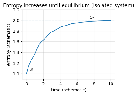

Entropy rises from $S_i$ to $S_f$ during a spontaneous process and then becomes constant at equilibrium.

A concrete example from Section 4.2 illustrates this. Two subsystems at different temperatures ($T_A > T_B$) in an insulated box exchange heat, and we showed that

as long as $T_A \neq T_B$. Energy flows from $A$ to $B$, raising $T_B$ and lowering $T_A$, until $T_A = T_B$. At that point the factor $(1/T_A - 1/T_B)$ vanishes, $dS = 0$, and the system has reached thermal equilibrium at the entropy maximum.

The Clausius Inequality¶

The entropy definition $dS = \delta q_{\mathrm{rev}}/T$ applies specifically to reversible heat transfer. A more general statement, valid for both reversible and irreversible processes, is the Clausius inequality:

• Equality holds for a reversible process: $dS = \delta q_{\mathrm{rev}}/T$.

• Strict inequality holds for an irreversible process: $dS > \delta q/T$.

The physical interpretation is that irreversibility produces additional entropy beyond the entropy “carried in” by heat flow. For an isolated system ($\delta q = 0$), the Clausius inequality reduces to $dS \ge 0$, recovering the second law.

The Clausius inequality also explains why the Carnot engine (Section 4.2) sets the maximum efficiency. Any irreversible engine operating between the same two reservoirs produces entropy internally ($dS_{\mathrm{irrev}} > 0$), so more heat must be rejected to the cold reservoir to compensate, reducing the net work output.

Entropy and the Number of Microstates: Boltzmann’s Formula¶

We now connect entropy to the microscopic picture. For an isolated system (microcanonical ensemble), the fundamental postulate of statistical mechanics (Section 2.1) assigns equal probability $p_i = 1/\Omega$ to each of the $\Omega$ accessible microstates. The entropy of such a system is

Here $\Omega$ is the number of microstates compatible with the macroscopic constraints (fixed $U$, $V$, $N$). You can think of $\Omega$ as the degeneracy of the macrostate: fix the total energy and other extensive quantities, then count how many distinct microscopic configurations share those values.

Why the Logarithm?¶

A key property of thermodynamic entropy is that it is extensive: for two independent subsystems $A$ and $B$,

But the number of microstates is multiplicative for independent systems:

The logarithm converts the product into a sum:

Without the logarithm, entropy would not be additive for independent subsystems.

Entropy in Terms of Probabilities: The Gibbs Entropy¶

The Gibbs (or Gibbs–Shannon) formula generalizes Boltzmann’s result from “counting equally likely microstates” to working with an arbitrary probability distribution $\{p_i\}$ over microstates $i = 1, \dots, M$:

This formula has two important features:

1. It reduces to Boltzmann’s formula in the microcanonical case. If all $\Omega$ accessible microstates are equally likely ($p_i = 1/\Omega$), then

   $$S = -k_{\mathrm{B}} \sum_{i=1}^{\Omega} \frac{1}{\Omega}\ln\!\left(\frac{1}{\Omega}\right) = -k_{\mathrm{B}}\ln\!\left(\frac{1}{\Omega}\right) = k_{\mathrm{B}}\ln\Omega.$$

   (9)

2. It applies when microstates are not equally likely — for instance, when the system is in contact with a heat bath (canonical ensemble). In this case, $p_i = e^{-\beta E_i}/Q$, and different microstates have different probabilities.

Canonical Ensemble: Entropy in Terms of the Partition Function¶

We now evaluate the Gibbs entropy for the canonical ensemble. Recall from Section 2.2 that a closed system (fixed $N$, $V$) in thermal contact with a reservoir at temperature $T$ has microstate probabilities

where the canonical partition function is

Derivation¶

Starting from the Gibbs entropy,

insert $\ln p_i = -\beta E_i - \ln Q$:

Using $\sum_i p_i = 1$ and the definition of internal energy from Section 2.3,

we obtain

Substituting $\beta = 1/(k_{\mathrm{B}} T)$:

This is a central result: it expresses the macroscopic state function $S$ directly in terms of the partition function $Q$ and the internal energy $U$, both of which we know how to compute from microscopic energy levels.

Connection to the Helmholtz Free Energy¶

Rearranging the boxed result gives

The left-hand side is the Helmholtz free energy, $A \equiv U - TS$ — a state function whose natural variables are $T$ and $V$. We therefore have

This result was foreshadowed in Section 2.3 (where it was stated as a Module 5 preview) and in Section 3.3 (where we noted that $A = U - TS$ would be “convenient at constant $T$ and $V$”). It is arguably the single most important equation in canonical statistical mechanics: if you can compute $Q$, you can compute $A$, and from $A$ you can derive all other thermodynamic quantities — $S$, $U$, $P$, $C_V$, and chemical potentials — by taking appropriate derivatives. We will develop this machinery in a later chapter.

Microscopic Interpretation of Heat (Connection to Section 3.2)¶

The results above connect naturally to the microscopic interpretation of the First Law developed in Section 3.2. Differentiating $U = \sum_i p_i E_i$ gives

For a closed system with only $PV$ work, comparing with $dU = \delta q + \delta w = \delta q - P\,dV$, we identified (Section 3.2):

• Heat: $\delta q = \sum_i E_i\, dp_i$ — energy exchange via redistributing probabilities among fixed energy levels.

• Work: $\delta w = \sum_i p_i\, dE_i$ — energy exchange via shifting the energy levels themselves (e.g., changing volume changes the particle-in-a-box levels).

The Gibbs entropy formula shows why this decomposition is natural. Since $S = -k_{\mathrm{B}}\sum_i p_i\ln p_i$ depends only on the probabilities $\{p_i\}$, entropy changes when and only when probabilities change — that is, when heat flows. Work, which shifts energy levels without redistributing probabilities, does not change the entropy. This is consistent with the macroscopic result: for a reversible adiabatic process ($\delta q = 0$), $dS = 0$.

Worked Examples¶

Example 1: Entropy of a two-state distribution¶

Problem. A system has two microstates with probabilities $p$ and $1-p$. Compute the Gibbs entropy and find where it is maximized.

Solution. The Gibbs entropy is

At $p = 1/2$ (maximally uncertain):

To confirm this is a maximum, note that $S(p)$ is concave (its second derivative $d^2S/dp^2 = -k_{\mathrm{B}}/[p(1-p)] < 0$ for $0 < p < 1$) and is zero at the endpoints $p = 0$ and $p = 1$, where one microstate has all the probability and there is no uncertainty.

Result. The maximum entropy $k_{\mathrm{B}}\ln 2$ occurs at $p = 1/2$, where the distribution is most spread out. This is consistent with Boltzmann’s formula: two equally likely microstates give $\Omega = 2$ and $S = k_{\mathrm{B}}\ln 2$.

Example 2: Entropy of the two-state system from Section 2.2¶

Problem. In Section 2.2, we analyzed a two-state system with energies $E_0 = 0$ and $E_1 = \varepsilon = 0.010\ \mathrm{eV}$ and found $p_0 = 0.596$ and $p_1 = 0.404$ at $T = 300\ \mathrm{K}$. Compute the entropy two ways: (a) from the Gibbs formula, and (b) from the canonical identity $S = U/T + k_{\mathrm{B}}\ln Q$.

Solution.

(a) Gibbs formula.

Evaluating: $0.596\ln(0.596) = -0.308$ and $0.404\ln(0.404) = -0.366$, so

(b) Canonical identity.

From Section 2.2: $Q = 1.679$, and $U = \varepsilon\,p_1 = (0.010)(0.404) = 4.04 \times 10^{-3}\ \mathrm{eV} = 6.47 \times 10^{-22}\ \mathrm{J}$.

Result. Both methods give the same answer, as they must — the canonical identity is derived from the Gibbs formula. Notice that the entropy ($0.674\,k_{\mathrm{B}}$) is less than the maximum ($k_{\mathrm{B}}\ln 2 = 0.693\,k_{\mathrm{B}}$) because the distribution is not perfectly uniform: the ground state is slightly more populated than the excited state at 300 K. At higher temperatures, the two probabilities would become more equal, and $S$ would approach $k_{\mathrm{B}}\ln 2$ from below.

Concept Checks¶

1. How does “entropy increases until equilibrium” translate into a statement about probability distributions over microstates?

2. Why does $S = k_{\mathrm{B}}\ln\Omega$ require the microcanonical assumption $p_i = 1/\Omega$? What goes wrong if you try to apply it to a canonical ensemble?

3. In the Gibbs entropy formula, why does $S = 0$ when $p_i = 1$ for one state and $p_j = 0$ for all others?

4. How can entropy be extensive (additive for independent subsystems) while probability distributions are normalized to 1?

5. Starting from $A = -k_{\mathrm{B}}T\ln Q$, how would you obtain $S$ and $U$ as functions of $T$? (Hint: think about which partial derivatives of $A$ give $S$ and $U$.)

Key Takeaways¶

• Entropy quantifies how many microstates — or how much probability weight — a macrostate contains.

• Boltzmann’s $S = k_{\mathrm{B}}\ln\Omega$ applies to isolated systems (microcanonical ensemble, equal probabilities). The logarithm ensures extensivity.

• The Gibbs formula $S = -k_{\mathrm{B}}\sum p_i\ln p_i$ generalizes Boltzmann’s result to any probability distribution and reduces to it in the microcanonical limit.

• In the canonical ensemble, $S = U/T + k_{\mathrm{B}}\ln Q$ ties entropy directly to the partition function.

• Rearranging gives the Helmholtz free energy $A = U - TS = -k_{\mathrm{B}}T\ln Q$ — the master potential from which all canonical thermodynamic quantities can be derived.

• The microscopic decomposition $dU = \sum p_i\,dE_i + \sum E_i\,dp_i$ (Section 3.2) is consistent with the entropy picture: only the $\sum E_i\,dp_i$ (heat) term changes probabilities and therefore changes entropy.