6.1. Phase Diagrams

Overview and Learning Objectives¶

In Section 5.1 we introduced the Gibbs free energy $G$ and showed that at constant $T$ and $P$ , a closed system moves spontaneously in the direction of decreasing $G$ and reaches equilibrium when $G$ is minimized. Section 5.3 closed by pointing out that this minimization principle also governs phase equilibria — the conditions under which a substance exists as solid, liquid, or gas, and the $(T,P)$ curves along which two phases coexist. That is the application we develop in this chapter.

A one-component substance at fixed $(T,P)$ can in principle exist in any of several phases, but only one is thermodynamically stable except on special curves in the $(T,P)$ plane where two (or at isolated points, three) phases coexist. These curves generate the familiar phase diagram. Our task in this section is to:

introduce the chemical potential $\mu$ as the open-system generalization of the Gibbs differential,
derive the phase-equilibrium condition $\mu_\alpha = \mu_\beta$ from the requirement that $G$ be minimized at fixed $T$ and $P$ , and
interpret that condition graphically on plots of $\bar g$ versus $T$ at fixed $P$ (and $\bar g$ versus $P$ at fixed $T$ ), and use it to identify the latent heat and entropy jump at a first-order phase transition.

The quantitative consequence of the equilibrium condition — the slope $dP/dT$ of a coexistence curve and its relation to the latent heat — is the Clapeyron equation, which we derive in Section 6.2.

Learning objectives:

Identify the key features of a one-component $P$ – $T$ phase diagram: single-phase regions, coexistence curves, triple point, and critical point.
Define the chemical potential $\mu_i$ as the open-system extension of $dG = -S\,dT + V\,dP$ , and recognize that for a pure substance $\mu = \bar g$ , the molar Gibbs free energy.
Derive the phase-equilibrium condition $\mu_\alpha = \mu_\beta$ from Gibbs minimization at fixed $T,P$ and interpret it as “no driving force for matter transfer.”
Read off the stable phase from intersecting $\bar g$ – $T$ or $\bar g$ – $P$ curves and relate the slopes to $-\bar s$ and $+\bar v$ .
Relate the latent heat and entropy jump at a first-order transition via $\Delta \bar h_{tr} = T_{tr}\,\Delta \bar s_{tr}$ , and use it together with Trouton’s rule to estimate $\Delta \bar s_{vap}$ from tabulated enthalpies of vaporization.

Core Ideas and Derivations¶

6.1.1 A quick tour of a one-component $P$ – $T$ phase diagram¶

A schematic $P$ – $T$ phase diagram for a single component contains regions where one phase is stable (solid, liquid, gas) separated by coexistence curves on which two phases are simultaneously in equilibrium.

Two special points deserve named attention:

Triple point (tp): the unique $(T_{tp},P_{tp})$ at which solid, liquid, and gas coexist simultaneously.
Critical point (cp): the point at which the liquid–gas coexistence curve terminates. Beyond the critical point, liquid and gas become indistinguishable and the system is called a supercritical fluid.

The critical point exists because liquid and gas differ only quantitatively — they are both disordered, fluid phases whose molar volumes can be made arbitrarily close to one another by heating the liquid and compressing the gas. Solid and liquid, by contrast, differ qualitatively (long-range translational order is either present or absent), so the solid–liquid line generally continues indefinitely as pressure increases rather than ending at a critical point.

Moving across a coexistence curve at fixed $P$ (or fixed $T$ ) changes which phase is thermodynamically stable — the defining feature of a phase transition. Our goal for the rest of this section is to characterize these transitions in terms of $G$ , and in particular to identify the condition that picks out the coexistence curves in the $(T,P)$ plane.

6.1.2 Open systems and the chemical potential¶

For a closed system at fixed composition, we derived in Section 5.1 the Gibbs differential

dG = -S\,dT + V\,dP.

(1)

A closed system cannot, however, describe two coexisting phases on its own, because at a phase transition matter is transferred from one phase to the other. To handle this, we regard each phase as a subsystem whose amount of matter can change. Each phase is then an open system — one that can exchange energy and matter with its surroundings (in this case, the other phase).

For an open, multicomponent system, the Gibbs differential generalizes to

dG = -S\,dT + V\,dP + \sum_i \mu_i\,dn_i,

(2)

where the sum runs over the chemical components $i$ and the chemical potential $\mu_i$ is defined by the partial derivative

\mu_i \equiv \left(\frac{\partial G}{\partial n_i}\right)_{T,P,\,n_{j\neq i}}.

(3)

In words: $\mu_i$ is how much the Gibbs free energy changes when one mole of component $i$ is added while holding $T$ , $P$ , and the amounts of all other components fixed. A “component” here means the minimum number of independent chemical species required to specify the composition of every phase in the system; for a pure substance the component count is one and there is a single chemical potential $\mu$ .

Picking up a thread from Chapter 5

In Section 5.1 we noted (in the dropdown “A curious consequence for $G$ ”) that holding $N$ fixed and applying the Euler relation gives the paradoxical result $G = 0$ for a one-component system, and promised to return to the issue once the chemical potential was in hand. With $\mu$ now defined, the resolution is immediate: the Euler relation for the Gibbs free energy of a one-component system is

G = \mu\,n,

(4)

so that the molar Gibbs free energy and the chemical potential are the same object:

\mu = \frac{G}{n} \equiv \bar g.

(5)

We use an overbar for molar quantities throughout this chapter ( $\bar g, \bar s, \bar v, \bar h$ ). For a pure substance, “chemical potential,” “molar Gibbs free energy,” and “ $G$ per mole” all refer to the same quantity, and we will use whichever name is most convenient.

Why $\mu$ , rather than $G$ itself, is the natural variable for phase equilibrium. The Gibbs free energy $G$ is extensive — it scales with the total amount of matter. The chemical potential is intensive: it depends on $T$ and $P$ but not on how much substance is present. This is precisely the property we need when asking “which of two phases is stable?” — a question whose answer should not depend on the size of the sample.

6.1.3 Phase equilibrium as “no driving force for matter transfer”¶

Consider a closed overall system containing two phases of the same pure substance, labeled $\alpha$ and $\beta$ , separated by a boundary across which matter can flow. Let the two phases hold $n_\alpha$ and $n_\beta$ moles respectively, with $n_\alpha + n_\beta = n_{\text{tot}}$ held fixed by overall matter conservation. Imagine transferring an infinitesimal amount $dn_\alpha$ from $\alpha$ to $\beta$ at fixed $T$ and $P$ ; then

dn_\beta = -dn_\alpha.

(6)

Applying the open-system Gibbs differential (2) to each phase and summing, and recognizing that at fixed $T$ and $P$ only the composition terms contribute,

dG = \mu_\alpha\,dn_\alpha + \mu_\beta\,dn_\beta = (\mu_\alpha - \mu_\beta)\,dn_\alpha.

(7)

At fixed $T$ and $P$ , the equilibrium condition is that $G$ be a minimum with respect to every internal variable, including the amount transferred. Requiring $dG = 0$ for arbitrary small transfers $dn_\alpha$ gives

\boxed{\mu_\alpha(T,P) = \mu_\beta(T,P)}.

(8)

This is the central result of Section 6.1: two phases of the same pure substance are in equilibrium at a given $(T,P)$ if and only if they have the same chemical potential.

The physical reading is that $\mu$ is the “price per mole” of adding substance to a phase. Matter spontaneously flows from higher $\mu$ to lower $\mu$ — from “expensive” to “cheap” — and stops flowing exactly when the two prices are equal. Away from equilibrium, the sign of $(\mu_\alpha - \mu_\beta)$ tells us which direction the transition runs:

If $\mu_\alpha > \mu_\beta$ , then $dG < 0$ when matter moves from $\alpha$ to $\beta$ , so the $\alpha \to \beta$ transition is spontaneous.
If $\mu_\alpha < \mu_\beta$ , the reverse transition is spontaneous.
If $\mu_\alpha = \mu_\beta$ , the two phases coexist at equilibrium.

Because $\mu$ depends on $T$ and $P$ , the equation $\mu_\alpha(T,P) = \mu_\beta(T,P)$ is a single scalar constraint on two variables and therefore picks out a curve in the $(T,P)$ plane — precisely the coexistence curve we saw in the phase diagram in Section 6.1.1.

6.1.4 Competing phases on $\bar g$ -vs- $T$ and $\bar g$ -vs- $P$ plots¶

The condition $\mu_\alpha = \mu_\beta$ becomes much more intuitive when we draw it graphically. For a pure substance, $\mu = \bar g$ , so a phase transition is the intersection of $\bar g$ -versus- $T$ (or $\bar g$ -versus- $P$ ) curves for the competing phases. The slopes of those curves encode entropy and volume via the Gibbs differential (1).

(A) $\bar g$ versus $T$ at fixed pressure¶

At constant pressure, Eq. (1) gives

\left(\frac{\partial \bar g}{\partial T}\right)_P = -\bar s.

(9)

On a $\bar g$ -vs- $T$ plot at fixed $P$ :

All phases have negative slope (entropy is positive).
The phase with the larger molar entropy has the more negative (steeper) slope.

Because typically $\bar s_g > \bar s_l > \bar s_s$ , the gas line is steepest, then liquid, then solid. Starting at low $T$ the solid curve is the lowest (most stable); as $T$ increases, the liquid curve eventually crosses the solid curve, and then the gas curve crosses the liquid. Each crossing marks a first-order phase transition at which the lowest- $\bar g$ phase — the stable one — changes.

(B) $\bar g$ versus $P$ at fixed temperature¶

At constant temperature, Eq. (1) gives

\left(\frac{\partial \bar g}{\partial P}\right)_T = \bar v.

(10)

On a $\bar g$ -vs- $P$ plot at fixed $T$ :

All phases have positive slope (molar volumes are positive).
The phase with the larger molar volume has the steeper slope.

Because typically $\bar v_g \gg \bar v_l \gtrsim \bar v_s$ , the gas line rises most steeply with pressure. Compressing the system therefore favors the phases with smaller molar volume (liquid or solid over gas) — the graphical statement of Le Châtelier’s principle for phase transitions. Water is the familiar counter-example on the solid–liquid side: because $\bar v_s > \bar v_l$ for water (ice is less dense than liquid water), the ice curve on a $\bar g$ -vs- $P$ plot rises faster than the liquid curve, so at fixed $T$ just below the normal freezing point, increasing $P$ can push the liquid below the solid and melt the ice.

In both views, the stable phase at each point is the one with the lowest $\bar g$ , and a phase transition occurs at each intersection. The graphical picture is particularly useful for understanding why the coexistence curves have the shapes they do — why increasing pressure generally raises melting and boiling points of normal substances, and why water’s ice–water line bends the “wrong” way.

6.1.5 Latent heat and entropy jump at a first-order transition¶

At most phase transitions (fusion, vaporization, sublimation, solid–solid polymorphic transitions) the first derivatives of $G$ — namely $S$ and $V$ — are discontinuous across the coexistence curve. Transitions of this kind are called first-order. The macroscopic consequences are two quantities that every student of thermodynamics encounters: a latent heat and an entropy jump.

For a transition $\alpha \to \beta$ occurring at $(T_{tr},P_{tr})$ , define the molar changes

\Delta \bar h_{tr} \equiv \bar h_\beta(T_{tr}) - \bar h_\alpha(T_{tr}), \qquad \Delta \bar s_{tr} \equiv \bar s_\beta(T_{tr}) - \bar s_\alpha(T_{tr}).

(11)

At the coexistence curve, $\mu_\alpha = \mu_\beta$ implies $\bar g_\alpha = \bar g_\beta$ and therefore $\Delta \bar g_{tr} = 0$ . Combined with $\Delta \bar g = \Delta \bar h - T\,\Delta \bar s$ , this gives the key identity

\boxed{\Delta \bar h_{tr} = T_{tr}\,\Delta \bar s_{tr}}.

(12)

Equation (12) connects a quantity one can measure calorimetrically — the latent heat $\Delta \bar h_{tr}$ , released or absorbed when matter crosses the boundary at constant pressure — to a quantity that usually appears only in tables, the entropy jump $\Delta \bar s_{tr}$ . It is the reason $\Delta \bar s_{vap}$ is rarely tabulated separately from $\Delta \bar h_{vap}$ : given one, the other follows by division.

Common special cases. At the melting temperature $T_{fus}$ (at the chosen pressure),

\Delta \bar h_{fus} = \bar h_l(T_{fus}) - \bar h_s(T_{fus}), \qquad \Delta \bar s_{fus} = \bar s_l(T_{fus}) - \bar s_s(T_{fus}),

(13)

and at the boiling temperature $T_{vap}$ ,

\Delta \bar h_{vap} = \bar h_g(T_{vap}) - \bar h_l(T_{vap}), \qquad \Delta \bar s_{vap} = \bar s_g(T_{vap}) - \bar s_l(T_{vap}).

(14)

Both are positive at ordinary first-order transitions: the higher-temperature phase is the one with greater molar enthalpy and greater molar entropy.

6.1.6 Trouton’s rule and water as an exception¶

Frederick Trouton (1884) noticed that for many ordinary liquids at their normal boiling point,

\Delta \bar s_{vap} \approx 85.9\ \mathrm{J\,mol^{-1}\,K^{-1}} \approx 10.3\,R.

(15)

The rough constancy of $\Delta \bar s_{vap}$ across chemically unrelated liquids suggests that the entropy cost of liberating one mole of molecules from a liquid into an ideal gas is governed mostly by the phase change itself — the volume increase, the loss of short-range order — rather than by the chemical identity of the liquid.

Real substances deviate from Trouton’s rule when the liquid is unusually ordered (hydrogen-bonded liquids such as water and the lower alcohols, metals with strong cohesion, liquid helium near its $\lambda$ -line). In these cases $\Delta \bar s_{vap}$ is larger than the Trouton value because the liquid is more ordered than an “average” liquid and correspondingly more entropy is gained on vaporization. Water is the familiar example: $\Delta \bar s_{vap}(\mathrm{H_2O}) \approx 109\ \mathrm{J\,mol^{-1}\,K^{-1}}$ , roughly 25 % above Trouton’s value, which is the macroscopic signature of hydrogen-bonding structure in liquid water. We will revisit the molecular interpretation of $\Delta \bar h_{vap}$ for water in Section 6.2 after introducing the Clausius–Clapeyron equation as a tool for extracting enthalpies of vaporization from vapor-pressure data.

Worked Example: Heating water from 298.15 K to 800 K at 1 bar¶

Goal. Estimate $\Delta \bar s$ and $\Delta \bar h$ when one mole of water is heated reversibly at constant pressure $P = 1$ bar from 298.15 K (liquid) to 800 K (superheated steam), crossing the liquid–vapor coexistence curve. This example combines the single-phase heating integrals developed in Chapters 3–4 with the first-order transition relation (12), and illustrates how strongly the overall entropy change is dominated by the phase transition itself.

Within a single phase at constant pressure,

\Delta \bar s = \int_{T_1}^{T_2} \frac{\bar c_P(T)}{T}\,dT, \qquad \Delta \bar h = \int_{T_1}^{T_2} \bar c_P(T)\,dT,

(16)

and at the coexistence temperature $T_{tr}$ the entropy has a finite jump

\Delta \bar s_{vap}(T_{tr}) = \frac{\Delta \bar h_{vap}(T_{tr})}{T_{tr}}.

(17)

We use a coarse set of $\bar c_P^{\,\circ}(T)$ values from the NIST–JANAF thermochemical tables for $\mathrm{H_2O(l)}$ and $\mathrm{H_2O(g)}$ at $P^\circ = 0.1\ \mathrm{MPa} = 1\ \mathrm{bar}$ . In that dataset, the liquid–vapor transition occurs at

T_{tr} = 372.780\ \mathrm{K}\quad\text{(very close to 373.15 K at 1 atm).}

(18)

Data used (excerpt)¶

Phase	$T$ (K)	$\bar c_P^{\,\circ}$ (J mol $^{-1}$ K $^{-1}$ )
$\mathrm{H_2O(l)}$	298.15	75.351
	300	75.349
	320	75.344
	340	75.388
	360	75.679
	372.780	75.962
$\mathrm{H_2O(g)}$	300	33.596
	400	34.262
	500	35.226
	600	36.325
	700	37.495
	800	38.721

The gas-phase heat capacity at $T_{tr}$ is obtained by linear interpolation of the 300–400 K JANAF entries. The latent heat at $T_{tr}$ is obtained from the tabulated standard enthalpies of formation:

\Delta \bar h_{vap}(T_{tr}) \approx \Delta_f H^\circ_g(T_{tr}) - \Delta_f H^\circ_l(T_{tr}).

(19)

import numpy as np

# ---- Cp(T) data (J/mol/K) ----
T_tr = 372.780  # K (liquid <-> vapor at 1 bar in the JANAF tables)

T_liq = np.array([298.15, 300, 320, 340, 360, T_tr])
Cp_liq = np.array([75.351, 75.349, 75.344, 75.388, 75.679, 75.962])

T_gas_tab = np.array([300, 400, 500, 600, 700, 800])
Cp_gas_tab = np.array([33.596, 34.262, 35.226, 36.325, 37.495, 38.721])

# Interpolate Cp_gas at T_tr (between 300 and 400 K)
Cp_gas_tr = Cp_gas_tab[0] + (T_tr - T_gas_tab[0])/(T_gas_tab[1] - T_gas_tab[0])*(Cp_gas_tab[1] - Cp_gas_tab[0])

T_gas = np.concatenate([[T_tr], T_gas_tab[1:]])
Cp_gas = np.concatenate([[Cp_gas_tr], Cp_gas_tab[1:]])

# ---- Heating contributions (trapezoid rule) ----
dS_liq = np.trapezoid(Cp_liq/T_liq, T_liq)          # J/mol/K
dH_liq = np.trapezoid(Cp_liq, T_liq)/1000           # kJ/mol

dS_gas = np.trapezoid(Cp_gas/T_gas, T_gas)          # J/mol/K
dH_gas = np.trapezoid(Cp_gas, T_gas)/1000           # kJ/mol

# ---- Vaporization jump from JANAF delta_f H° (linear interpolation to T_tr) ----
# liquid delta_f H° at 360 and 400 K (kJ/mol)
Hf_liq_360, Hf_liq_400 = -283.874, -282.591
Hf_liq_tr = Hf_liq_360 + (T_tr-360)/(400-360)*(Hf_liq_400 - Hf_liq_360)

# gas delta_f H° at 300 and 400 K (kJ/mol)
Hf_gas_300, Hf_gas_400 = -241.844, -242.846
Hf_gas_tr = Hf_gas_300 + (T_tr-300)/(400-300)*(Hf_gas_400 - Hf_gas_300)

dH_vap = Hf_gas_tr - Hf_liq_tr                 # kJ/mol
dS_vap = dH_vap*1000/T_tr                      # J/mol/K

print(f"Heating (liquid, 298.15 -> {T_tr:.3f} K):  ΔH = {dH_liq:6.3f} kJ/mol,  ΔS = {dS_liq:6.2f} J/mol/K")
print(f"Vaporization at {T_tr:.3f} K (1 bar):        ΔH = {dH_vap:6.2f} kJ/mol,  ΔS = {dS_vap:6.2f} J/mol/K")
print(f"Heating (gas,    {T_tr:.3f} -> 800 K):       ΔH = {dH_gas:6.2f} kJ/mol,  ΔS = {dS_gas:6.2f} J/mol/K")

dH_total = dH_liq + dH_vap + dH_gas
dS_total = dS_liq + dS_vap + dS_gas
print(f"\nTOTAL (298.15 K liquid -> 800 K steam, 1 bar): ΔH ≈ {dH_total:6.2f} kJ/mol,  ΔS ≈ {dS_total:6.1f} J/mol/K")

Heating (liquid, 298.15 -> 372.780 K):  ΔH =  5.633 kJ/mol,  ΔS =  16.87 J/mol/K
Vaporization at 372.780 K (1 bar):        ΔH =  40.89 kJ/mol,  ΔS = 109.69 J/mol/K
Heating (gas,    372.780 -> 800 K):       ΔH =  15.48 kJ/mol,  ΔS =  27.57 J/mol/K

TOTAL (298.15 K liquid -> 800 K steam, 1 bar): ΔH ≈  62.01 kJ/mol,  ΔS ≈  154.1 J/mol/K

What to notice. The total entropy change along this path is dominated by the phase transition: $\Delta \bar s_{vap} \approx 1.1\times 10^2\ \mathrm{J\,mol^{-1}\,K^{-1}}$ , which alone is several times the combined contribution of heating the liquid by ~75 K and the vapor by ~430 K. Water’s large $\Delta \bar s_{vap}$ relative to Trouton’s value (15) is the macroscopic signature of hydrogen-bonding structure in the liquid, consistent with the discussion in Section 6.1.6.

import matplotlib.pyplot as plt

# Cumulative entropy relative to 298.15 K along the path (trapezoid segments)
S_liq_cum = np.concatenate([[0.0], np.cumsum(0.5*(Cp_liq[1:]/T_liq[1:] + Cp_liq[:-1]/T_liq[:-1]) * np.diff(T_liq))])
S_gas_cum = np.concatenate([[0.0], np.cumsum(0.5*(Cp_gas[1:]/T_gas[1:] + Cp_gas[:-1]/T_gas[:-1]) * np.diff(T_gas))])

T_path = np.concatenate([T_liq, T_gas[1:]])
S_path = np.concatenate([S_liq_cum, S_liq_cum[-1] + dS_vap + S_gas_cum[1:]])

plt.figure()
plt.plot(T_path, S_path)
plt.axvline(T_tr, linestyle="--")
plt.xlabel("Temperature (K)")
plt.ylabel(r"$\Delta \bar s$ from 298.15 K (J mol$^{-1}$ K$^{-1}$)")
plt.title("Heating water at 1 bar: entropy rise + vaporization jump")
plt.show()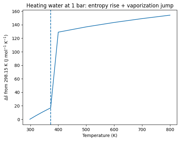

The sharp vertical step at $T_{tr}$ is the graphical signature of a first-order transition: a finite entropy jump at a single temperature, sitting atop a smooth continuous rise from heat-capacity integration through each single-phase region.

Concept Checks¶

Why is the chemical potential, rather than the Gibbs free energy itself, the natural variable for analyzing phase equilibria?
On a $\bar g$ -vs- $T$ plot at fixed pressure, what does the slope of each curve represent, and why do different phases have different slopes? Use your answer to predict the order of the solid, liquid, and gas slopes.
Starting from $\mu_\alpha = \mu_\beta$ at coexistence, argue in words why this condition defines a curve in the $(T,P)$ plane rather than an isolated point or a two-dimensional region. What happens when a third phase is added to the argument?
Water has $\Delta \bar s_{vap} \approx 109\ \mathrm{J\,mol^{-1}\,K^{-1}}$ , about 25 % higher than Trouton’s value. What does this tell you about the liquid relative to an “average” liquid? (Nothing yet about the gas.)
Ice floats on water, so $\bar v_s > \bar v_l$ for water. On a $\bar g$ -vs- $P$ plot at fixed $T$ just below the normal freezing point, sketch the ice and water curves and identify which has the steeper slope. What does your sketch predict for the effect of increasing $P$ on the stable phase at that temperature?

Key Takeaways¶

For an open system, the Gibbs differential acquires a composition term: $dG = -S\,dT + V\,dP + \sum_i \mu_i\,dn_i$ . The chemical potential $\mu_i \equiv (\partial G/\partial n_i)_{T,P,n_{j\neq i}}$ is the intensive quantity conjugate to amount of substance, and for a pure substance $\mu = \bar g$ .
Two phases of a pure substance are in equilibrium if and only if they have equal chemical potentials: $\mu_\alpha(T,P) = \mu_\beta(T,P)$ . Because this is a single constraint on two variables, it defines the coexistence curve in the $(T,P)$ plane.
The stable phase at a given $(T,P)$ is the one with the lowest $\bar g$ . On $\bar g$ – $T$ plots (fixed $P$ ) and $\bar g$ – $P$ plots (fixed $T$ ), the slopes are $-\bar s$ and $+\bar v$ respectively; intersections mark first-order phase transitions.
At a first-order transition, the latent heat and entropy jump are tied together by $\Delta \bar h_{tr} = T_{tr}\,\Delta \bar s_{tr}$ .
Trouton’s rule, $\Delta \bar s_{vap} \approx 85.9\ \mathrm{J\,mol^{-1}\,K^{-1}}$ at the normal boiling point, is a useful benchmark; water exceeds it because of hydrogen-bonding order in the liquid.
The slope $dP/dT$ of a coexistence curve — the quantitative statement of how a phase boundary bends through the $(T,P)$ plane — is the subject of Section 6.2.