6.2. Clapeyron and Clausius–Clapeyron

Course-wide Conventions & Notation

Overview and Learning Objectives¶

In Section 6.1 we showed that two phases of a pure substance are in equilibrium at a given $(T,P)$ if and only if their chemical potentials are equal:

Because this is a single scalar constraint on two variables, it picks out a curve in the $(T,P)$ plane — the coexistence curve we saw in the phase diagram. What it does not immediately give us is the slope $dP/dT$ of that curve, which is what we would need to predict, for instance, how a boiling point shifts with pressure or how a vapor pressure changes with temperature.

In this section we differentiate the equilibrium condition along the coexistence curve to obtain the Clapeyron equation, a general expression for $dP/dT$ that applies to any first-order phase transition. We then specialize it to the liquid–vapor case under two further approximations — the gas molar volume dominates, and the vapor is ideal — to obtain the Clausius–Clapeyron equation, which is the working tool for analyzing vapor-pressure data.

Learning objectives:

• Differentiate $\mu_\alpha(T,P) = \mu_\beta(T,P)$ along a coexistence curve to derive the Clapeyron equation $dP/dT = \Delta\bar s/\Delta\bar v = \Delta\bar h_{tr}/(T\,\Delta\bar v)$.

• Apply the Clapeyron equation to ice → water and explain physically why the solid–liquid coexistence curve for water has a negative slope, in contrast to most substances.

• Apply the approximations $\bar v_g \gg \bar v_l$ and $\bar v_g = RT/P$ to obtain the differential Clausius–Clapeyron equation $d\ln P / dT = \Delta\bar h_{vap}/(RT^2)$.

• Integrate the Clausius–Clapeyron equation under the constant-$\Delta\bar h_{vap}$ approximation and use a two-point dataset to estimate $\Delta\bar h_{vap}$ from vapor-pressure measurements.

• Diagnose the failure of the constant-$\Delta\bar h_{vap}$ assumption from residuals of a $\ln P$-vs-$1/T$ fit, and use a local-slope estimate to recover $\Delta\bar h_{vap}(T)$.

Core Ideas and Derivations¶

6.2.1 The Clapeyron equation¶

Pick a point $(T,P)$ on a coexistence curve between phases $\alpha$ and $\beta$, and consider an infinitesimal displacement $(dT,dP)$ that stays on the curve. By construction, the equilibrium condition continues to hold along the curve, so $\mu_\alpha$ and $\mu_\beta$ change by equal amounts:

For a one-component, single-phase system, the Gibbs differential per mole reads

which is just the molar form of $dG = -S\,dT + V\,dP$ specialized to a pure substance (so that $\mu = \bar g$, as established in Section 6.1.2). Apply Eq. (3) to each phase along the coexistence curve:

Collecting $dT$ and $dP$ terms,

and using the entropy–latent-heat relation $\Delta\bar h_{tr} = T\,\Delta\bar s_{tr}$ derived in Section 6.1.5, we obtain the Clapeyron equation:

Three things to notice about Eq. (6):

1. It is exact. No approximation has been made beyond the assumption that the transition is first-order (so $\Delta\bar v$ and $\Delta\bar h$ are well-defined finite jumps) and that both phases are pure.

2. The sign of $dP/dT$ is set by the sign of $\Delta\bar v$, since $\Delta\bar h$ and $T$ are positive for any “normal” transition (the higher-temperature phase is the higher-enthalpy one). Most substances have $\bar v_l > \bar v_s$ at the melting line and $\bar v_g \gg \bar v_l$ at the boiling line, so both slopes are positive — an increase in pressure raises both the melting and the boiling temperature.

3. The magnitude of $dP/dT$ is set by $\Delta\bar v$. Solid–liquid transitions have very small $\Delta\bar v$ and consequently very steep coexistence curves; liquid–vapor transitions have very large $\Delta\bar v$ and consequently shallow coexistence curves. This is the reason why melting points are nearly insensitive to ordinary pressure changes while boiling points are very sensitive.

6.2.2 Worked example: melting of ice and the negative-slope coexistence curve¶

Water is the textbook exception to “$\bar v_l > \bar v_s$”: ice floats on liquid water because $\bar v_s > \bar v_l$ near the normal melting point. By Eq. (6), this forces the slope of the ice–water coexistence curve to be negative.

Inputs (at $T_{fus} = 273.15$ K, $P = 1$ bar):

• $\Delta\bar h_{fus} = 6.010\ \text{kJ mol}^{-1}$

• $\rho_s = 0.917\ \text{g cm}^{-3}$, $\rho_l = 0.9998\ \text{g cm}^{-3}$

• $M(\mathrm{H_2O}) = 18.015\ \text{g mol}^{-1}$

Molar volumes of the two phases:

The molar volume decreases on melting:

Clapeyron slope. Insert into Eq. (6):

Physical interpretation. Inverting the slope gives $dT/dP \approx -7.4\ \text{mK bar}^{-1}$: increasing the pressure on ice by one bar lowers its melting point by about seven thousandths of a kelvin. Even at 100 bar — well above any pressure encountered in everyday situations — the melting point depression is only about 0.74 K. This is enough to let the ice–water phase boundary bend perceptibly to the left on the phase diagram, but it is far too small to account for the popular “pressure melting” explanation of ice skating, where contact pressures of a few hundred bar would depress $T_{fus}$ by at most a degree or two (skating works mainly because of friction-generated heating and a thin pre-existing surface liquid layer, not pressure melting).

6.2.3 The Clausius–Clapeyron equation (liquid–vapor with ideal vapor)¶

For the liquid–vapor coexistence curve, the molar-volume change is overwhelmingly dominated by the gas:

(For water at the normal boiling point, $\bar v_g \approx 3.0\times 10^{-2}\ \text{m}^3\,\text{mol}^{-1}$ versus $\bar v_l \approx 1.9\times 10^{-5}\ \text{m}^3\,\text{mol}^{-1}$ — a ratio of more than 10³, so dropping $\bar v_l$ introduces an error of less than 0.1%.)

If we further approximate the vapor as an ideal gas at the saturation pressure,

then the Clapeyron equation (6) becomes

Dividing both sides by $P_{sat}$ and recognizing $d\ln P_{sat} = dP_{sat}/P_{sat}$ gives the Clausius–Clapeyron equation in differential form:

The quadratic $T^{-2}$ dependence — rather than the $T^{-1}$ that one might naively expect — is a direct consequence of having used $\bar v_g = RT/P$ in the Clapeyron equation: one factor of $T$ comes from the explicit $T$ in the denominator of Clapeyron, and the other from the $RT$ in $\bar v_g$.

Integrated form (constant $\Delta \bar h_{vap}$ approximation)¶

If $\Delta\bar h_{vap}$ varies only weakly with $T$ over the range of interest, it can be pulled outside the integral:

so that

Two algebraically equivalent rearrangements of Eq. (16) are useful for different purposes:

• For two known $(T,P)$ points, solve for the unknown $\Delta\bar h_{vap}$:

  $$\Delta\bar h_{vap} = R\,\frac{\ln(P_2/P_1)}{(1/T_1 - 1/T_2)}.$$

  (17)

• For fitting a dataset, recognize that taking $\ln$ of Eq. (16) and treating one of the points as a reference gives

  $$\ln P_{sat}(T) = -\frac{\Delta\bar h_{vap}}{R}\,\frac{1}{T} + \text{const.}$$

  (18)

  A plot of $\ln P_{sat}$ versus $1/T$ should be a straight line with slope $-\Delta\bar h_{vap}/R$ — provided the constant-$\Delta\bar h_{vap}$ approximation actually holds.

6.2.4 Worked example: estimating $\Delta\bar h_{vap}$ of water from two vapor-pressure points¶

Use the integrated Clausius–Clapeyron form (17) to estimate $\Delta\bar h_{vap}$ for water given the following two points on its saturation curve:

• $T_1 = 363.15\ \text{K}$ (90 °C), $P_1 = 70.12\ \text{kPa}$

• $T_2 = 373.15\ \text{K}$ (100 °C, normal boiling point), $P_2 = 101.325\ \text{kPa}$ (1 atm)

Both points are taken from the NIST WebBook saturation tables for water.

Step 1. Compute the logarithm of the pressure ratio:

Step 2. Compute the inverse-temperature factor:

Step 3. Combine using Eq. (17):

Discussion. The two-point estimate of $41.5\ \text{kJ mol}^{-1}$ sits a few percent above the calorimetric value $\Delta\bar h_{vap}(\text{H}_2\text{O}, 100\,°\text{C}) = 40.66\ \text{kJ mol}^{-1}$. The discrepancy is not just measurement noise: it reflects the fact that $\Delta\bar h_{vap}$ is itself slightly temperature-dependent (it decreases with rising $T$ and vanishes at the critical point), so an estimate built from data points spanning 90–100 °C produces an average over that interval rather than the value at the upper endpoint. We will return to the temperature dependence of $\Delta\bar h_{vap}$ in the mini-lab below.

A molecular reading of the result¶

Why is $\Delta\bar h_{vap}$ for water of order 40 kJ mol$^{-1}$? The molecular interpretation gives a satisfying back-of-the-envelope answer that ties the macroscopic measurement to Chapter 2’s stat-mech picture of intermolecular interactions. In liquid water, each molecule participates on average in roughly two hydrogen bonds (each H-bond is shared between two molecules), and a single hydrogen bond is worth $\sim 20\ \text{kJ mol}^{-1}$. Vaporizing one mole of water to an effectively non-interacting gas therefore costs roughly

in striking agreement with experiment. The estimate is rough — it omits dispersion interactions and treats each H-bond as an isolated bond — but it captures the right order of magnitude and identifies the dominant physics. The same argument explains the large value of $\Delta\bar s_{vap}$ for water and its deviation from Trouton’s rule (Section 6.1.6): the liquid is more ordered than an “average” liquid because of its hydrogen-bonded structure, so vaporization releases more entropy as well as more enthalpy.

Mini-lab: Vapor pressure → $\Delta\bar h_{vap}$, linearity limits, and $\Delta\bar h_{vap}(T)$¶

Goals¶

1. Use a Clausius–Clapeyron plot to estimate an average $\Delta\bar h_{vap}$ from a vapor-pressure dataset.

2. Diagnose when the straight-line model breaks down by examining residuals.

3. Estimate a temperature-dependent $\Delta\bar h_{vap}(T)$ from local slopes of the same data.

Dataset: saturation vapor pressure of water¶

Use this dataset as if it were experimental measurements (the values are smooth and consistent, so they are good for analysis practice rather than for assessing experimental uncertainty).

Part A. Global Clausius–Clapeyron fit (the “straight-line” model)¶

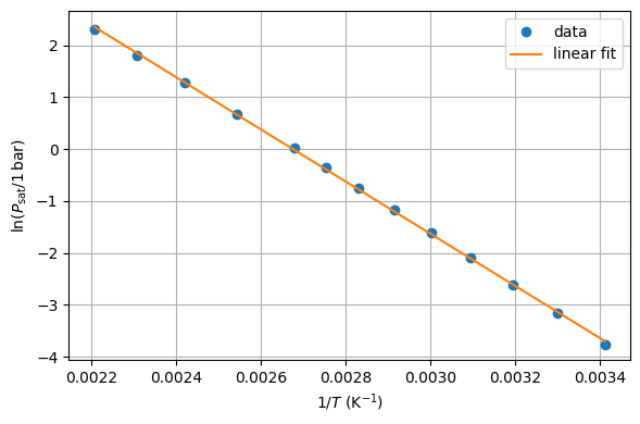
Task. Plot $y = \ln(P_{sat}/1\ \text{bar})$ versus $x = 1/T$ (with $T$ in K), fit a line, and extract $\Delta\bar h_{vap}$ from the slope.

import io
import numpy as np
import pandas as pd
import matplotlib.pyplot as plt
from scipy import stats

R = 8.314462618  # J mol^-1 K^-1

data = """T_C,P_kPa
20,2.3296
30,4.2317
40,7.3584
50,12.3056
60,19.8702
70,31.0872
80,47.2671
90,70.0298
100,101.3365
120,197.9718
140,358.9652
160,613.6815
180,997.4430
"""

df = pd.read_csv(io.StringIO(data))
df["T_K"] = df["T_C"] + 273.15
df["P_bar"] = df["P_kPa"] / 100.0  # 100 kPa = 1 bar
df["invT"] = 1.0 / df["T_K"]
df["lnP"] = np.log(df["P_bar"])    # ln(P/1 bar)

# Linear regression: lnP = m*(1/T) + b
m, b, r, p, se = stats.linregress(df["invT"], df["lnP"])
DeltaHvap = -m * R  # J/mol

print(f"slope m            = {m:10.2f} K")
print(f"intercept b        = {b:10.3f}")
print(f"R^2                = {r**2:10.6f}")
print(f"DeltaHvap (global) = {DeltaHvap/1000:10.2f} kJ/mol")

# Plot
x = df["invT"].to_numpy()
y = df["lnP"].to_numpy()
x_fit = np.linspace(x.min(), x.max(), 200)
y_fit = m*x_fit + b

plt.figure(figsize=(6,4))
plt.plot(x, y, "o", label="data")
plt.plot(x_fit, y_fit, "-", label="linear fit")
plt.xlabel(r"$1/T\ (\mathrm{K^{-1}})$")
plt.ylabel(r"$\ln(P_\mathrm{sat}/1\,\mathrm{bar})$")
plt.grid(True)
plt.legend()
plt.tight_layout()
plt.show()

slope m            =   -5028.86 K
intercept b        =     13.456
R^2                =   0.999666
DeltaHvap (global) =      41.81 kJ/mol

Interpretation prompts (one or two sentences each):

• What units should $\Delta\bar h_{vap}$ have, and how do they emerge from the slope formula?

• Why is the slope of $\ln P_{sat}$ versus $1/T$ negative?

• Does the line look straight over the full temperature range?

Part B. Linearity limits: residuals beat “it looks straight”¶

A Clausius–Clapeyron plot can look linear by eye even when the constant-$\Delta\bar h_{vap}$ assumption is quietly failing. A quick diagnostic is a residual plot.

df["lnP_fit"] = m*df["invT"] + b
df["residual"] = df["lnP"] - df["lnP_fit"]

plt.figure(figsize=(6,4))
plt.axhline(0, linewidth=1)
plt.plot(df["invT"], df["residual"], "o-")
plt.xlabel(r"$1/T\ (\mathrm{K^{-1}})$")
plt.ylabel("residual = data − fit (in ln units)")
plt.grid(True)
plt.tight_layout()
plt.show()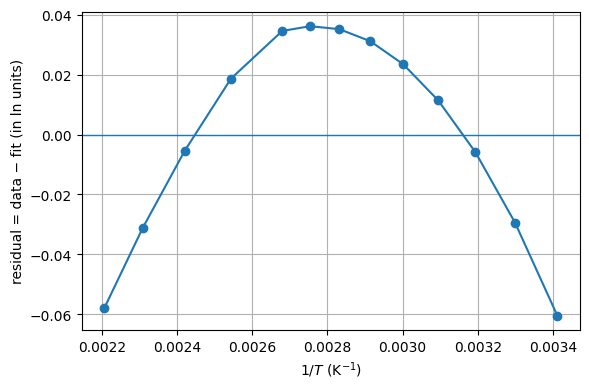

What to look for:

• Random scatter around zero → the linear model is adequate over this range.

• A systematic curve (e.g. negative at both ends, positive in the middle, or vice versa) → the straight-line model is missing physics, most likely because $\Delta\bar h_{vap}(T)$ is changing with $T$ across the dataset.

Part C. Two-range fits: do you get the same $\Delta\bar h_{vap}$?¶

If $\Delta\bar h_{vap}$ were truly constant, then fitting two separate temperature subranges should give the same slope within uncertainty. If they disagree systematically, that is hard evidence that $\Delta\bar h_{vap}$ depends on $T$.

def fit_subset(df_sub):
    m, b, r, p, se = stats.linregress(df_sub["invT"], df_sub["lnP"])
    return {
        "T_range_C": (df_sub["T_C"].min(), df_sub["T_C"].max()),
        "R2": round(r**2, 6),
        "DeltaHvap_kJmol": round((-m*R)/1000, 2),
    }

low  = df[df["T_C"].between(20, 90)]
high = df[df["T_C"].between(120, 180)]

print("Low-T  fit:", fit_subset(low))
print("High-T fit:", fit_subset(high))

Low-T  fit: {'T_range_C': (np.int64(20), np.int64(90)), 'R2': np.float64(0.999927), 'DeltaHvap_kJmol': np.float64(43.02)}
High-T fit: {'T_range_C': (np.int64(120), np.int64(180)), 'R2': np.float64(0.99999), 'DeltaHvap_kJmol': np.float64(39.92)}

Part D. A “local slope” estimate of $\Delta\bar h_{vap}(T)$¶

From the differential form (14),

so we can estimate $\Delta\bar h_{vap}(T)$ from finite differences of the $(T,\ln P_{sat})$ data.

T = df["T_K"].to_numpy()
lnP = df["lnP"].to_numpy()

# central differences for d(lnP)/dT
dlnP_dT = np.empty_like(T)
dlnP_dT[1:-1] = (lnP[2:] - lnP[:-2]) / (T[2:] - T[:-2])
dlnP_dT[0]    = (lnP[1] - lnP[0]) / (T[1] - T[0])
dlnP_dT[-1]   = (lnP[-1] - lnP[-2]) / (T[-1] - T[-2])

df["DeltaHvap_local_kJmol"] = (R * T**2 * dlnP_dT) / 1000

plt.figure(figsize=(6,4))
plt.plot(df["T_C"], df["DeltaHvap_local_kJmol"], "o-")
plt.xlabel(r"$T\ (^\circ\mathrm{C})$")
plt.ylabel(r"local $\Delta\bar h_\mathrm{vap}(T)$ (kJ/mol)")
plt.grid(True)
plt.tight_layout()
plt.show()

df[["T_C","DeltaHvap_local_kJmol"]]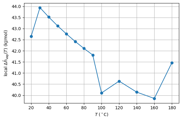

Loading...

Interpretation. The local $\Delta\bar h_{vap}(T)$ should decrease monotonically with increasing temperature. Physically, as $T$ rises toward the critical point, the liquid and vapor phases become more and more similar in density and structure, so the molar enthalpy difference between them shrinks. At the critical point itself, $\Delta\bar h_{vap}\to 0$ — there is no longer a meaningful “vaporization” because the two phases have merged.

Reflection questions¶

1. Over what temperature window does the Clausius–Clapeyron straight-line model look “good enough” and have residuals that are roughly random?

2. List two physical reasons why $\ln P$ versus $1/T$ might curve over a wider range.

3. If you needed a better model than a single $\Delta\bar h_{vap}$, what would you do? (Examples: fit two ranges, use a published vapor-pressure correlation such as Antoine’s equation, or include the temperature dependence of $\Delta\bar h_{vap}$ via heat-capacity corrections.)

Computational Studio: Clausius–Clapeyron¶

Interact with real vapor-pressure data for ethanol. The studio transforms the dataset to visualize the Clausius–Clapeyron linearization ($\ln P$ versus $1/T$), lets you dynamically adjust the regression bounds to explore linearity limits, and reports the corresponding $\Delta\bar h_{vap}$ extracted from the slope.

You can open the studio in a new tab: Clausius–Clapeyron Studio.

Concept Checks¶

1. Why does $d\ln P/dT$ in the Clausius–Clapeyron equation depend on $1/T^2$ rather than simply on $1/T$? Trace the two factors of $T$ back to the steps of the derivation.

2. What is the sign of $dP/dT$ for the ice → water transition, and what specific feature of the molar volumes is responsible for that sign? Contrast with the corresponding transition for a “normal” substance such as benzene.

3. Why is it usually safe to approximate $\Delta\bar v \approx \bar v_g$ for vaporization but not for melting?

4. The local-slope analysis in Part D of the mini-lab shows $\Delta\bar h_{vap}(T)$ decreasing as $T$ rises. Explain qualitatively what would happen to $d\ln P/dT$ — and to the apparent slope of a $\ln P$-versus-$1/T$ plot — if you were to extend the dataset all the way up to the critical point.

5. A student fits a Clausius–Clapeyron line to vapor-pressure data and extracts $\Delta\bar h_{vap} = 38\ \text{kJ mol}^{-1}$ for a polar liquid that should give around 45 kJ mol$^{-1}$ from calorimetry. List two distinct error sources that could be responsible.

Key Takeaways¶

• Differentiating the equilibrium condition $\mu_\alpha = \mu_\beta$ along a coexistence curve produces the Clapeyron equation $dP/dT = \Delta\bar s_{tr}/\Delta\bar v_{tr} = \Delta\bar h_{tr}/(T\,\Delta\bar v_{tr})$, which is exact for any first-order transition between pure phases.

• The sign of $dP/dT$ is set by the sign of $\Delta\bar v$. For water, $\bar v_s > \bar v_l$ at the melting line, so the ice–water coexistence curve has a negative slope ($\sim -135$ bar K$^{-1}$).

• For liquid–vapor equilibrium with $\bar v_g \gg \bar v_l$ and an ideal vapor, the Clapeyron equation specializes to the Clausius–Clapeyron equation $d\ln P_{sat}/dT = \Delta\bar h_{vap}/(RT^2)$.

• Under the constant-$\Delta\bar h_{vap}$ approximation, the integrated Clausius–Clapeyron equation gives $\ln(P_2/P_1) = -(\Delta\bar h_{vap}/R)(1/T_2 - 1/T_1)$, which extracts $\Delta\bar h_{vap}$ from two vapor-pressure points or from a linear fit of $\ln P_{sat}$ versus $1/T$.

• Deviations from a straight line in $\ln P_{sat}$ versus $1/T$ — best diagnosed from residuals, not by eye — signal the breakdown of the constant-$\Delta\bar h_{vap}$ approximation. A local-slope analysis recovers the temperature-dependent $\Delta\bar h_{vap}(T)$ and shows it falling toward zero at the critical point.

• For water, $\Delta\bar h_{vap} \approx 40\ \text{kJ mol}^{-1}$ is consistent with the molecular picture of breaking roughly two hydrogen bonds per molecule on going from liquid to vapor — the macroscopic shadow of the intermolecular interactions developed in Chapter 2.